Walking Randomly

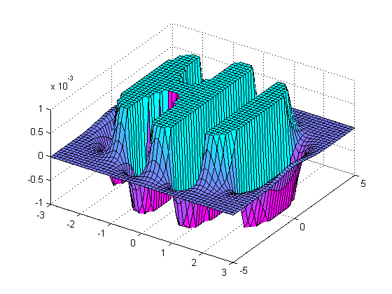
One of the earliest posts I made on Walking Randomly (almost 3 years ago now – how time flies!) described the following equation and gave a plot of it in Mathematica.

Some time later I followed this up with another blog post and a Wolfram Demonstration.

Well, over at Stack Overflow, some people have been rendering this cool equation using MATLAB. Here’s the first version

x = linspace(-3,3,50);
y = linspace(-5,5,50);
[X Y]=meshgrid(x,y);
Z = exp(-X.^2-Y.^2/2).*cos(4*X) + exp(-3*((X+0.5).^2+Y.^2/2));
Z(Z>0.001)=0.001;
Z(Z<-0.001)=-0.001;
surf(X,Y,Z);
colormap(flipud(cool))
view([1 -1.5 2])

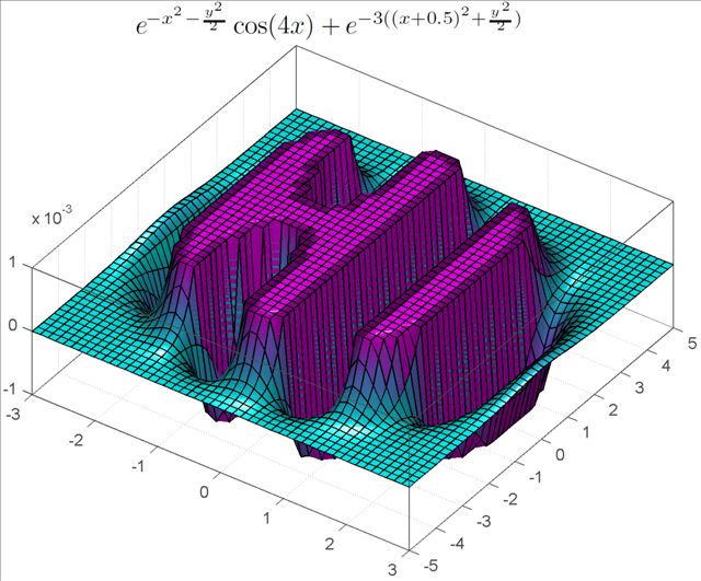
and here’s the second.

[x y] = meshgrid( linspace(-3,3,50), linspace(-5,5,50) );
z = exp(-x.^2-0.5*y.^2).*cos(4*x) + exp(-3*((x+0.5).^2+0.5*y.^2));
idx = ( abs(z)>0.001 );
z(idx) = 0.001 * sign(z(idx)); 

figure('renderer','opengl')
patch(surf2patch(surf(x,y,z)), 'FaceColor','interp');
set(gca, 'Box','on', ...
    'XColor',[.3 .3 .3], 'YColor',[.3 .3 .3], 'ZColor',[.3 .3 .3], 'FontSize',8)
title('$e^{-x^2 - \frac{y^2}{2}}\cos(4x) + e^{-3((x+0.5)^2+\frac{y^2}{2})}$', ...
    'Interpreter','latex', 'FontSize',12) 

view(35,65)
colormap( [flipud(cool);cool] )
camlight headlight, lighting phong

Do you have any cool graphs to share?

Over at Mathrecreation, Dan Mackinnon has been plotting two dimensional polygonal numbers on quadratic number spirals using a piece of software called Fathom. Today’s train-journey home project for me was to reproduce this work using Mathematica and Python.

I’ll leave the mathematics to Mathrecreation and Numberspiral.com and just get straight to the code. Here’s the Mathematica version:

• Download the Mathematica Notebook
• Download a fully interactive version that will run on the free Mathematica Player

p[k_, n_] := ((k - 2) n (n + 1))/2 - (k - 3) n;
Manipulate[
 nums = Table[p[k, n], {n, 1, numpoints}];
 If[showpoints,
  ListPolarPlot[Table[{2*Pi*Sqrt[n], Sqrt[n]}, {n, nums}]
   , Joined -> joinpoints, Axes -> False,
   PlotMarkers -> {Automatic, Small}, ImageSize -> {400, 400}],
  ListPolarPlot[Table[{2*Pi*Sqrt[n], Sqrt[n]}, {n, nums}]
   , Joined -> joinpoints, Axes -> False, ImageSize -> {400, 400}
   ]
  ]
 , {k, 2, 50, Appearance -> "Labeled"}
 , {{numpoints, 100, "Number of points"}, {100, 250, 500}}
 , {{showpoints, True, "Show points"}, {True, False}}
 , {{joinpoints, True, "Join points"}, {True, False}}
 , SaveDefinitions :> True
 ]

A set of 4 screenshots is shown below (click the image for a higher resolution version). The formula for polygonal numbers, p(kn,n), is only really valid for integer k and so I made a mistake when I allowed k to be any real value in the code above. However, I liked some of the resulting spirals so much that I decided to leave the mistake in.

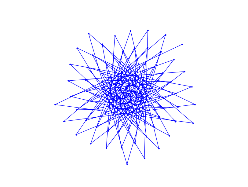
When Dan showed the images he produced from Fathom, he mentioned that he would one day like to implement these systems in a more open platform. Well, you can’t get much more open than Python so here’s a piece of code that makes use of Python and the matplotlib package (download the file – polygonal_spiral.py).

#!/usr/bin/env python
import matplotlib.pyplot as plt
from math import *
 
def p(k,n):
   return(((k-2)*n*(n+1))/2 -(k-3)*n)
 
k=13
 
polygonal_nums = [p(k,n) for n in range(100)]
theta = [2*pi*sqrt(n) for n in polygonal_nums]
r = [sqrt(n) for n in polygonal_nums]
 
myplot = plt.polar(theta,r,'.-')
plt.gca().axis('off')
plt.show()

Now, something that I haven’t figured out yet is why the above python code works just fine for 100 points but if you increase it to 101 then you just get a single point. Does anyone have any ideas?

Unlike my Mathematica version, the above Python program does not give you an interactive GUI but I’ll leave that as an exercise for the reader.

If you enjoyed this post then you might also like:

• Simulating Harmonographs
• Quadraflakes,Pentaflakes,Hexaflakes and more

A Mathematica user recently asked me if I could help him speed up the following Mathematica code. He has some data and he wants to model it using the following model

dFIO2 = 0.8;
PBH2O = 732;
dCVO2[t_] := 0.017 Exp[-4 Exp[-3 t]];
dPWO2[t_?NumericQ, v_?NumericQ, qL_?NumericQ, q_?NumericQ] := 
 PBH2O*((v/(v + qL))*dFIO2*(1 - E^((-(v + qL))*t)) + 
    q*NIntegrate[E^((v + qL)*(\[Tau] - t))*dCVO2[\[Tau]], {\[Tau], 0, t}])

Before starting to apply this to his actual dataset, he wanted to check out the performance of the NonlinearModelFit[] command. So, he created a completely noise free dataset directly from the model itself

data = Table[{t, dPWO2[t, 33, 25, 55]}, {t, 0, 6, 6./75}];

and then, pretending that he didn’t know the parameters that formed that dataset, he asked NonlinearModelFit[] to find them:

fittedModel = NonlinearModelFit[data, dPWO2[t, v, qL, q], {v, qL, q}, t]; // Timing
params = fittedModel["BestFitParameters"]

On my machine this calculation completes in 11.21 seconds and gives the result we expect:

{11.21, Null} 
{v -> 33., qL-> 25., q -> 55.} 

11.21 seconds is too slow though since he wants to evaluate this on real data many hundreds of times. How can we make it any faster?

I started off by trying to make NIntegrate go faster since this will be evaluated potentially hundreds of times by the optimizer. Turning off Symbolic pre-processing did the trick nicely in this case. To turn off Symbolic pre-processing you just add

Method -> {Automatic, "SymbolicProcessing" -> 0}

to the end of the NIntegrate command. So, we re-define his model function as

dPWO2[t_?NumericQ, v_?NumericQ, qL_?NumericQ, q_?NumericQ] := 
 PBH2O*((v/(v + qL))*dFIO2*(1 - E^((-(v + qL))*t)) + 
    q*NIntegrate[E^((v + qL)*(\[Tau] - t))*dCVO2[\[Tau]], {\[Tau], 0, t}
,Method -> {Automatic, "SymbolicProcessing" -> 0}])

This speeds things up almost by a factor of 2.

fittedModel = NonlinearModelFit[data, dPWO2[t, v, qL, q], {v, qL, q}, t]; // Timing
params = fittedModel["BestFitParameters"]

{6.13, Null}
{v -> 33., qL -> 25., q -> 55.}

Not bad but can we do better?

Giving Mathematica a helping hand.

Like most optimizers, NonlinearModelFit[] will work a lot faster if you give it a decent starting guess. For example if we provide a close-ish guess at the starting parameters then we get a little more speed

fittedModel = 
   NonlinearModelFit[data, 
    dPWO2[t, v, qL, q], {{v, 25}, {qL, 20}, {q, 40}}, 
    t]; // Timing
params = fittedModel["BestFitParameters"]

{5.78, Null}
{v -> 33., qL -> 25., q -> 55.}

give an even better starting guess and we get yet more speed

fittedModel = 
   NonlinearModelFit[data, 
    dPWO2[t, v, qL, q], {{v, 31}, {qL, 24}, {q, 54}}, 
    t]; // Timing
params = fittedModel["BestFitParameters"]

{4.27, Null}
{v -> 33., qL -> 25., q -> 55.}

Ask the audience

So, that’s where we are up to so far. Neither of us have much experience with this particular part of Mathematica so we are hoping that someone out there can speed this calculation up even further. Comments are welcomed.

On a Linux machine with a normal install of Mathematica you can usually get access to a command line version of Mathematica by typing

math

at the command line.  Command line Mathematica is useful for situations where you want to do batch processing, perhaps as part of a Condor pool or something, but I’ll not write about that until another time.

On a Mac, however, a standard install of Mathematica doesn’t give you a math command so you have to create it yourself.  Add the following line to your system’s /etc/bashrc file.

alias math="/Applications/Mathematica.app/Contents/MacOS/MathKernel"

Now, when you type math at the command prompt it will behave just like a Linux system which is sometimes useful.

Someone recently emailed me to say that they thought Mathematica sucked because it couldn’t integrate abs(x) where abs stands for absolute value.  The result he was expecting was

When you try to do this in Mathematica 7.0.1, it appears that it simply can’t do it. The command

Integrate[Abs[x], x]

just returns the integral unevaluated

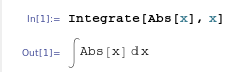
I’ve come across this issue before and many people assume that Mathematica is just stupid…after all it appears that it can’t even do an integral expected of a high school student. Well, the issue is that Mathematica is not a high school student and it assumes that x is a complex variable. For complex x, this indefinite integral doesn’t have a solution!

So, let’s tell Mathematica that x is real

Integrate[Abs[x], x, Assumptions :> Element[x, Reals]]

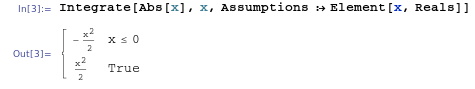
which is Mathematica’s way of saying that the answer is -x^2/2 for x<=0 and x^2/2 otherwise, i.e. when x>0. It’s not quite in the form we were originally expecting but a moments thought should convince you that they are the same thing.

Interestingly, it seems that Wolfram Alpha guesses that you probably mean real x since it just evaluates the integral of abs(x) directly. It does, however, give the result in yet another form: in terms of the signum function, sgn(x):

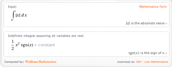
A couple of weeks ago I am pretty sure that Wolfram Alpha gave exactly the same result as Mathematica 7.0.1 so I wonder if they have quietly upgraded the back-end Kernel of Wolfram Alpha.  Perhaps this is how Mathematica version 8 will evaluate this result?

Ever since version 6 of Mathematica was released (way back in 2007) I have received dozens of queries from users at my University saying something along the lines of ‘Plotting no longer works in Mathematica’ or ‘If I wrap my plot in a Do loop then I get no output.  The user usually goes on to say that it worked perfectly well in pre-v6 versions of Mathematica, is clearly a bug and could I please file a bug report with Wolfram Research?

It’s not a bug….it’s a feature!

If you have googled your way here and just want a fast solution to your problem then here goes.  I assume that you have code that looks like this

Do[
 Plot[Cos[n x], {x, -Pi, Pi}]
 , {n, 1, 3}
 ]

and you were expecting to get a set of nice plots (in this case 3) – one plot for each iteration of your loop. Instead, Mathematica 6 or above is giving you nothing…nada…zip! There are several ways you can ‘fix’ this and I am going to show you two. Option 1 is to wrap your Plot Command with Print

Do[
 Print[Plot[Cos[n x], {x, -Pi, Pi}]]
 , {n, 1, 3}
 ]

Option 2 is to use Table instead of Do

Table[
 Plot[Cos[n x], {x, -Pi, Pi}]
 , {n, 1, 3}
 ]

I am imaging that the average googler has now disappeared having got what they came for but some of you are possibly wondering why the above two ‘fixes’ work.  Here’s my attempt at an explanation.

Old versions of Mathematica (v5.2 and below) treated graphics very differently to the way that Mathematica works today. The output of a command such as Plot[] used to contain two parts – the first was a Graphics object which looked a bit like the following in the notebook front end

– Graphics –

This was the OutputForm of the actual symbolic result of the Plot[] command. The second part – the actual visualization of the plot – was effectively just a side effect that happened to be what us humans actually wanted.

In version 6 and above, the OutputForm of a Graphics object is its visualisation which makes a lot more sense then just – Graphics –. The practical upshot of this is that there is now no need for a ‘side effect’ since the visualization of the plot IS the output.  If you are confused then this bit is explained much more eloquently in an old Wolfram Blog post.

That’s the first part of the story regarding plots in loops.  The second piece of the puzzle is to know that when you wrap a Mathematica expression in a Do loop then you suppress its output but you don’t suppress any side effects.  In version 5.2 the plot is a side effect and so it gets displayed on each iteration of the loop.  In version 6 and above, the plot is the output and so gets suppressed unless you explicitly ask for it to be displayed using Print[].

Does this help clear things up?  Comments welcomed.

I recently received a notification about the 2010 International Mathematica Symposium (IMS) which is due to take place in Beijing, China from July 16th this year.  The IMS is not run by Wolfram Research (although I think that Wolfram is a sponsor) but is run by Mathematica enthusiasts for Mathematica enthusiasts.  I was lucky enough to be able to attend both the 2008 IMS in Maastricht and the 2006 IMS in Avignon where I had a fantastic time, learned lots of stuff and met loads of people who just love Mathematica and mathematics.

I have to say that I have never been to a conference quite like the IMS before; the attendees were simply fizzing with enthusiasm and the range of talks and activities were wonderful.  In Avignon, I learned how to use Manipulate even before Mathematica 6 was released.  In Maastrict I was among the first to see some of the new features in Mathematica 7 and have seen Mathematica applied to subject areas as diverse as cancer research, high school math teaching, puzzle solving, quantum mechanics, electronics, radio astronomy and finance.  I’ve been taught Mathematica tricks from some of the very people who wrote the thing and have swapped programming methods and scripts with users of all levels.

The knowledge base of those attending the IMS ranges from people who eat, breathe and sleep Mathematica through to people who have only just started using it and everything in between.  I’ve met (and now consider among my friends) a statistics expert from Australia, a genetic algorithms expert from Canada and a college instructor from Finland among many others.  I’ve celebrated Mathematica’s 20th birthday in some underground caves, had my head read and also got a couple of very nice T-shirts which I love but my wife refuses to be seen with (she doesn’t like my MATLAB T-shirts either)!

There is usually a sprinkling of Wolfram employees among the attendees which gives you the chance to get the inside track on what is going on within Wolfram Research.  If you have a problem understanding something in Mathematica or there is a bug that winds you up then who better to talk to?  The IMS has also given me the chance to meet the authors of some of the most well known Mathematica books over the years which was fantastic.  Discussing a fun math problem with people like this and then watching them cook up a cool looking demonstration in minutes will surely get your imagination fired up.

Unfortunately, due to a distinct lack of funds, I probably won’t be at the IMS in Beijing but if you are into Mathematica and can make it there then I highly suggest you go.  You won’t regret it and I’d appreciate it if someone could send me the T-Shirt ;)

Regular readers of Walking Randomly will know that I am a big fan of the Manipulate function in Mathematica.  Manipulate allows you to easily create interactive mathematical demonstrations for teaching, research or just plain fun and is the basis of the incredibly popular Wolfram Demonstrations Project.

Sage, probably the best open source mathematics software available right now, has a similar function called interact and I have been playing with it a bit recently (see here and here) along with some other math bloggers.  The Sage team have done a fantastic job with the interact function but it is missing a major piece of functionality in my humble opinion – a Locator control.

In Mathematica the default control for Manipulate is a slider:

Manipulate[Plot[Sin[n x], {x, -Pi, Pi}], {n, 1, 10}]

The slider is also the default control for Sage’s interact:

@interact
def _(n=(1,10)):
    plt=plot(sin(n*x),(x,-pi,pi))
    show(plt)

Both systems allow the user to use other controls such as text boxes, checkboxes and dropdown menus but Mathematica has a control called a Locator that Sage is missing.  Locator controls allow you to directly interact with a plot or graphic.  For example, the following Mathematica code (taken from its help system) draws a polygon and allows the user to click and drag the control points to change its shape.

Manipulate[Graphics[Polygon[pts], PlotRange -> 1],
 {{pts, {{0, 0}, {.5, 0}, {0, .5}}}, Locator}]

The Locator control has several useful options that allow you to customise your demonstration even further. For example, perhaps you want to allow the user to move the vertices of the polygon but you don’t want them to be able to actually see the control points. No problem, just add Appearance -> None to your code and you’ll get what you want.

Manipulate[Graphics[Polygon[pts], PlotRange -> 1],
 {{pts, {{0, 0}, {.5, 0}, {0, .5}}}, Locator, Appearance -> None}]

Another useful option is LocatorAutoCreate -> True which allows the user to create extra control points by holding down CTRL and ALT (or just ALT – it depends on your system it seems) as they click in the active area.

Manipulate[Graphics[Polygon[pts], PlotRange -> 1],
 {{pts, {{0, 0}, {.5, 0}, {0, .5}}}, Locator,
  LocatorAutoCreate -> True}]

When you add all of this functionality together you can do some very cool stuff with just a few lines of code. Theodore Gray’s curve fitting code on the Wolfram Demonstrations project is a perfect example.

All of these features are demonstrated in the video below

So, onto the bounty hunt.  I am offering 25 pounds worth (about 40 American Dollars) of books from Amazon to anyone who writes the code to implement a Locator control for Sage’s interact function.  To get the prize your code must fulfil the following spec

• Your code must be accepted into the Sage codebase and become part of the standard install.  This should ensure that it is of reasonable quality.
• There should be an option like Mathematica’s LocatorAutoCreate -> True to allow the user to create new locator points interactively by Alt-clicking (or via some other suitable method).
• There should be an option to alter the appearance of the Locator control (e.g. equivalent to Mathematica’s Appearance -> x option).  As a minimum you should be able to do something like Appearance->None
• You should provide demonstration code that implements everything shown in the video above.
• I have to be happy with it!

And the details of the prize:

• I only have one prize – 25 pounds worth of books (about 40 American dollars) from Amazon.  If more than one person claims it then the prize will be split.
• The 25 pounds includes whatever it will cost for postage and packing.
• I won’t send you the voucher – I will send you the books of your choice as a ‘gift’.  This will mean that you’ll have to send me your postal address. Don’t enter if this bothers you for some reason.
• I expect you to be sensible regarding the exact value of the prize.  So if your books come to 24.50 then we’ll call it even.  Similarly if they come to 25.50 then I won’t argue.
• I am not doing this on behalf of any organisation.  It’s my personal money.
• My decision is final and I can withdraw this prize offer at any time without explanation.  I hope you realise that I am just covering my back by saying this – I have every intention of giving the prize but whenever money is involved one always worries about the possibility of being ripped off.

Good luck!

Update (29th December 2009): The bounty hunt has only been going for a few days and the bounty has already doubled to 50 pounds which is around 80 American dollars.  Thanks to David Jones for his generosity.

There was a discussion recently on comp.soft-sys.math.mathematica about maintaining a user-led Mathematica bug list and various solutions were proposed.  I have no desire (and certainly no time) to even try to maintain a ‘proper’ bug database for Mathematica but I am interested in maintaining a list of bugs that I personally find interesting and that I would like to see explained or fixed.

This post is that list.

First – some answers to potential questions.

Why are you doing this?  I thought you liked Mathematica.

I love Mathematica but, like all pieces of software, it is not perfect.  I find (some of) the imperfections interesting and since I get lots of hits from google every month from people looking for bugs in MATLAB, Mathematica, Maple, Mathcad etc then I assume that I am not alone.  Every bug that I discuss here will be submitted to Wolfram Research and I will also update the page when the bug gets fixed.

I emailed/wrote a comment about a bug and you haven’t included it in the list. Why?

Sorry about that – please don’t take it personally.  I am low on time and may not have managed to verify the ‘bug’ or maybe it just didn’t tickle my fancy.  It’s also possible that I simply don’t understand the problem you are referring to and I will not post anything on here that I don’t at least think I understand.  Remember – I’m not trying to keep a list of all Mathematica bugs – just some of the ones that I find interesting.

One of the ‘bugs’ you posted is not a bug – you just misunderstood the situation.

Oops, sorry!  Please educate me so I can update it.

I think I have found a bug in Mathematica – what should I do?

In the first instance I suggest you post it to comp.soft-sys.math.mathematica – there are plenty of people there who know a lot about Mathematica and they (probably) will let you know if you really have found a bug or not. If everyone suspects that it is a bug then your next step is to report it to Wolfram.  Finally, if you think I’d like to know about it then feel free to leave a comment to this post or email me.

FullSimplify bug 1

Clear[n];
FullSimplify[n Exp[-n * 0.], Element[n, Integers]]

expected output:

n

actual output:

n/2

original source – here.

Integrate bug 1

Integrate[k^2 (k^2 - 1)/((k^2 - 1)^2 + x^2)^(3/2), {k, 0, Infinity},Assumptions -> x > 0]

Expected output:

1/2*1/(1+x^2)^(1/4)*EllipticK(1/2*2^(1/2)*(((1+x^2)^(1/2)+1)/(1+x^2)^(1/2))^(1/2))

Actual output:

EllipticK[(2*x)/(-I + x)]/(2*Sqrt[-1 - I*x])

Note that although the integrand is real for all k, Mathematica gives a complex result which is clearly wrong.  Original source – here.

Limit bug 1

Limit[EllipticTheta[3, 0, x], x -> 1, Direction -> 1]

Expected Output:

Infinity

Actual Output:

0

Original Source: here

NetworkFlow bug

The following code should complete in less than a second.

<< "Combinatorica`"
NetworkFlow[CompleteGraph[4, 4], 1, 8]

but in Mathematica 7.0.1 (tested on Windows and Linux) it never completes and hogs a CPU indefinitely. Wolfram are aware of this one and it should be fixed in the next release. Thanks to Gábor Megyesi of Manchester University for sending me this one.

Feel free to let me know of others that you find but please bear in mind the points at the beginning of this post.

Earlier today I was chatting to a lecturer over coffee about various mathematical packages that he might use for an upcoming Masters course  (note – offer me food or drink and I’m happy to talk about pretty much anything). He was mainly interested in Mathematica and so we spent most of our time discussing that but it is part of my job to make sure that he considers all of the alternatives – both commercial and open source. The course he was planning on running (which I’ll keep to myself out of respect for his confidentiality) was definitely a good fit for Mathematica but I felt that SAGE might suite him nicely as well.

“Does it have nice, interactive functionality like Mathematica’s Manipulate function?” he asked

Oh yes! Here is a toy example that I coded up in about the same amount of time that it took to write the introductory paragraph above (but hopefully it has no mistakes). With just a bit of effort pretty much anyone can make fully interactive mathematical demonstrations using completely free software. For more examples of SAGE’s interactive functionality check out their wiki.

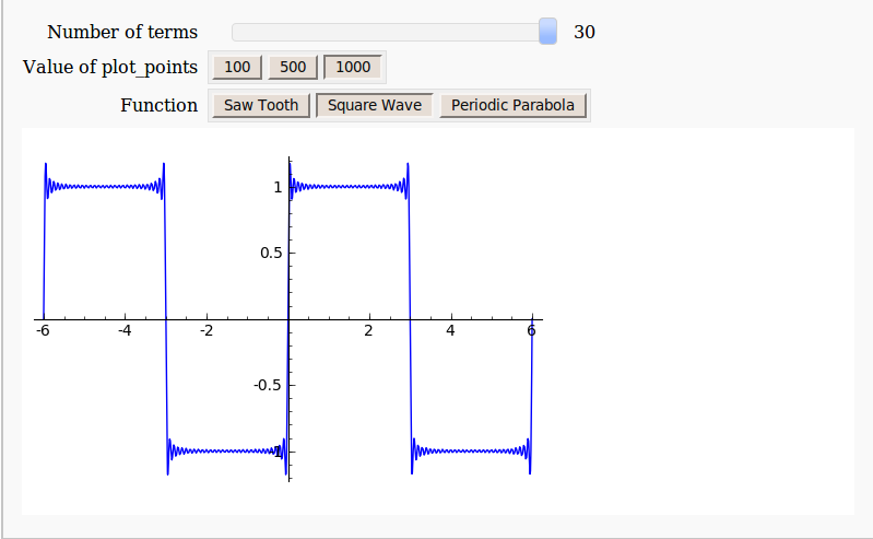
Here’s the code:

def ftermSquare(n):
 return(1/n*sin(n*x*pi/3))

def ftermSawtooth(n):
 return(1/n*sin(n*x*pi/3))

def ftermParabola(n):
 return((-1)^n/n^2 * cos(n*x))

def fseriesSquare(n):
 return(4/pi*sum(ftermSquare(i) for i in range (1,2*n,2)))

def fseriesSawtooth(n):
 return(1/2-1/pi*sum(ftermSawtooth(i) for i in range (1,n)))

def fseriesParabola(n):
 return(pi^2/3 + 4*sum(ftermParabola(i) for i in range(1,n)))

@interact
def plotFourier(n=slider(1, 30,1,10,'Number of terms')
,plotpoints=('Value of plot_points',[100,500,1000]),Function=['Saw Tooth','Square Wave','Periodic Parabola']):
    if Function=='Saw Tooth':
     show(plot(fseriesSawtooth(n),x,-6,6,plot_points=plotpoints))
    if Function=='Square Wave':
     show(plot(fseriesSquare(n),x,-6,6,plot_points=plotpoints))
    if Function=='Periodic Parabola':
     show(plot(fseriesParabola(n),x,-6,6,plot_points=plotpoints))