
Archive for the ‘programming’ Category
The MATLAB community site, MATLAB Central, is celebrating its 20th anniversary with a coding competition where the only aim is to make an interesting image with under 280 characters of code. The 280 character limit ensures that the resulting code is tweetable. There are a couple of things I really like about the format of this competition, other than the obvious fact that the only aim is to make something pretty!
- No MATLAB license is required! Sign up for a free MathWorks account and away you go. You can edit and run code in the browser.
Stealingreusing other people’s code is actively encouraged! The competition calls it remixing but GitHub users will recognize it as forking.
Here’s an example. I wrote a piece of code to render the Sierpiński triangle – Wikipedia using a simple random algorithm called the Chaos game.
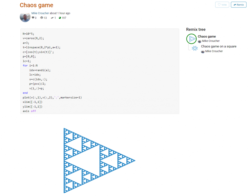
This is about as simple as the Chaos game gets and there are many things that could be done to produce a different image. As you can see from the Remix tree on the right hand side, I’ve already done one of them by changing a from 3 to 4 and adding some extra code to ensure that the same vertex doesn’t get chosen twice. This is result:
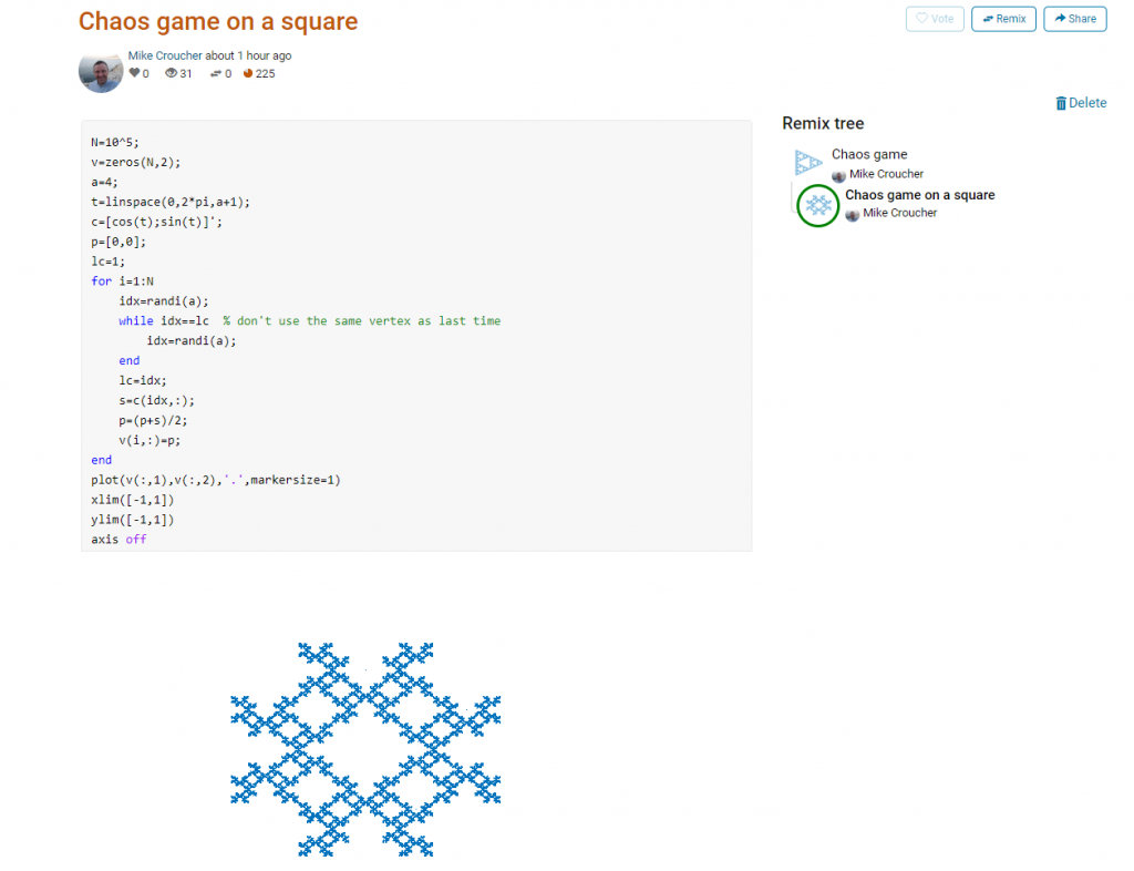
Someone else can now come along, hit the remix button and edit the code to produce something different again. Some things you might want to try for the chaos game include
- Try changing the value of a which is used in the variables t and c to produce the vertices of a polygon on an enclosing circle.
- Instead of just using the vertices of a polygon, try using the midpoints or another scheme for producing the attractor points completely.
- Try changing the scaling factor — currently p=(p+s)/2;
- Try putting limitations on which vertex is chosen. This remix ensures that the current vertex is different from the last one chosen.
- Each vertex is currently equally likely to be chosen using the code idx=randi(a); Think of ways to change the probabilities.
- Think of ways to colorize the plots.
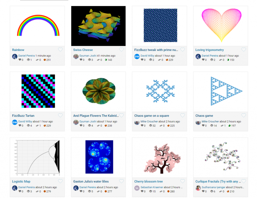
Maybe the chaos game isn’t your thing. You are free to create your own design from scratch or perhaps you’d prefer to remix some of the other designs in the gallery.
The competition is just a few hours old and there are already some very nice ideas coming out.
Feel free to discuss and contribute to this article over at the corresponding GitHub repo.
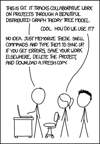
Many people suggest that you should use version control as part of your scientifc workflow. This is usually quickly followed up by recommendations to learn git and to put your project on GitHub. Learning and doing all of this for the first time takes a lot of effort. Alongside all of the recommendations to learn these technologies are horror stories telling how difficult it can be and memes saying that no one really knows what they are doing!
There are a lot of reasons to not embrace the git but there are even more to go ahead and do it. This is an attempt to convince you that it’s all going to be worth it alongside a bunch of resources that make it easy to get started and academic papers discussing the issues that version control can help resolve.
This document will not address how to do version control but will instead try to answer the questions what you can do with it and why you should bother. It was inspired by a conversation on twitter.
Improvements to individual workflow
Ways that git and GitHub can help your personal computational workflow – even if your project is just one or two files and you are the only person working on it.
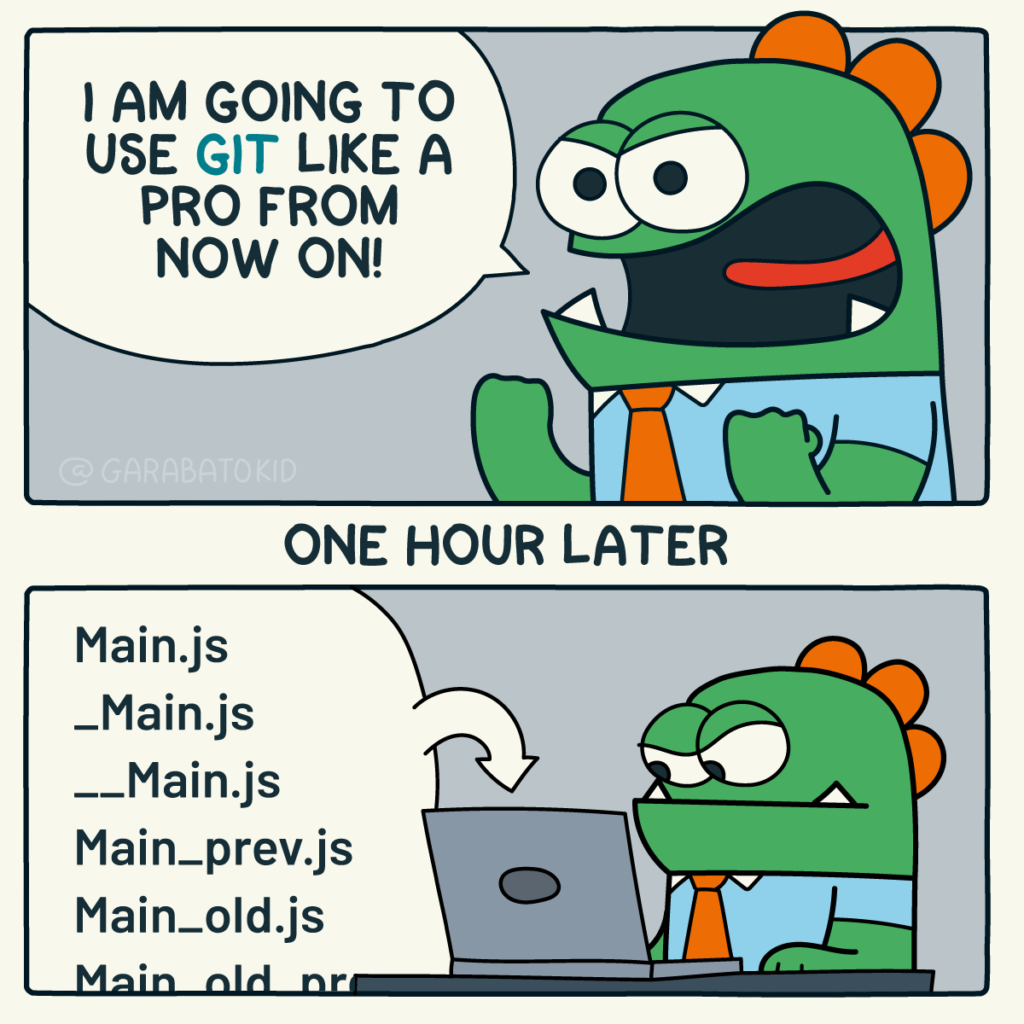
Fixing filename hell
Is this a familiar sight in your working directory?
mycode.py
mycode_jane.py
mycode_ver1b.py
mycode_ver1c.py
mycode_ver1b_january.py
mycode_ver1b_january_BROKEN.py
mycode_ver1b_january_FIXED.py
mycode_ver1b_january_FIXED_for_supervisor.py
For many people, this is just the beginning. For a project that has existed long enough there might be dozens or even hundreds of these simple scripts that somehow define all of part of your computational workflow. Version control isn’t being used because ‘The code is just a simple script developed by one person’ and yet this situation is already becoming the breeding ground for future problems.
- Which one of these files is the most up to date?
- Which one produced the results in your latest paper or report?
- Which one contains the new work that will lead to your next paper?
- Which ones contain deep flaws that should never be used as part of the research?
- Which ones contain possibly useful ideas that have since been removed from the most recent version?
Applying version control to this situation would lead you to a folder containing just one file
mycode.pyAll of the other versions will still be available via the commit history. Nothing is ever lost and you’ll be able to effectively go back in time to any version of mycode.py you like.
A single point of truth
I’ve even seen folders like the one above passed down generations of PhD students like some sort of family heirloom. I’ve seen labs where multple such folders exist across a dozen machines, each one with a mixture of duplicated and unique files. That is, not only is there a confusing mess of files in a folder but there is a confusing mess of these folders!
This can even be true when only one person is working on a project. Perhaps you have one version of your folder on your University HPC cluster, one on your home laptop and one on your work machine. Perhaps you email zipped versions to yourself from time to time. There are many everyday events that can lead to this state of affairs.
By using a GitHub repository you have a single point of truth for your project. The latest version is there. All old versions are there. All discussion about it is there.
Everything…one place.
The power of this simple idea cannot be overstated. Whenever you (or anyone else) wants to use or continue working on your project, it is always obvious where to go. Never again will you waste several days work only to realise that you weren’t working on the latest version.
Keeping track of everything that changed
The latest version of your analysis or simulation is different from the previous one. Thanks to this, it may now give different results today compared to yesterday. Version control allows you to keep track of everything that changed between two versions. Every line of code you added, deleted or changed is highlighted. Combined with your commit messages where you explain why you made each set of changes, this forms a useful record of the evolution of your project.
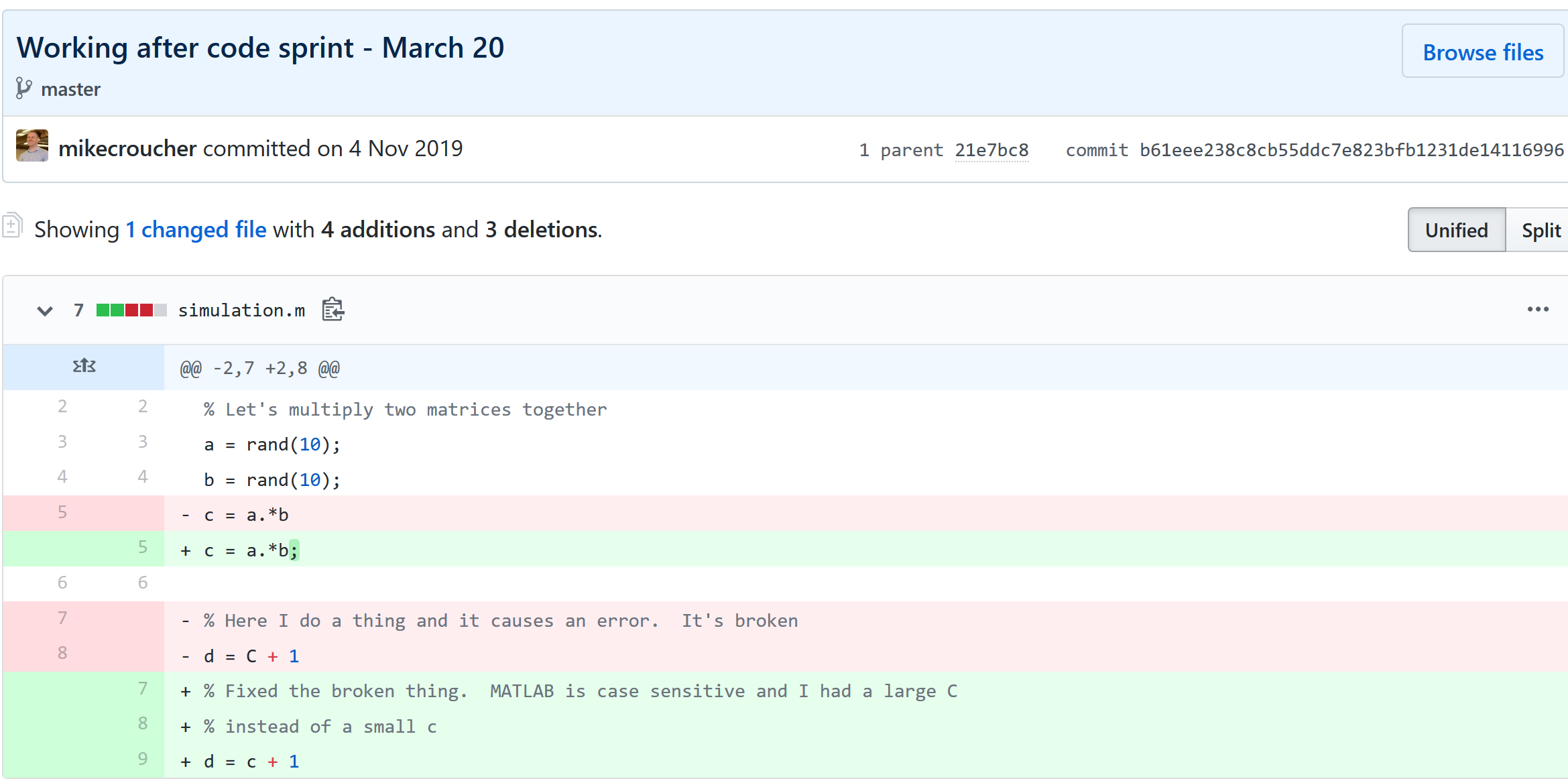
It is possible to compare the differences between any two commits, not just two consecutive ones which allows you to track the evolution of your project over time.
Always having a working version of your project
Ever noticed how your collaborator turns up unnanounced just as you are in the middle of hacking on your code. They want you to show them your simulation running but right now its broken! You frantically try some of the other files in your folder but none of them seem to be the version that was working last week when you sent the report that moved your collaborator to come to see you.
If you were using version control you could easily stash your current work, revert to the last good commit and show off your work.
Tracking down what went wrong
You are always changing that script and you test it as much as you can but the fact is that the version from last year is giving correct results in some edge case while your current version is not. There are 100 versions between the two and there’s a lot of code in each version! When did this edge case start to go wrong?
With git you can use git bisect to help you track down which commit started causing the problem which is the first step towards fixing it.

Providing a back up of your project
Try this thought experiment: Your laptop/PC has gone! Fire, theft, dead hard disk or crazed panda attack.

It, and all of it’s contents have vanished forever. How do you feel? What’s running through your mind? If you feel the icy cold fingers of dread crawling up your spine as you realise Everything related to my PhD/project/life’s work is lost then you have made bad life choices. In particular, you made a terrible choice when you neglected to take back ups.
Of course there are many ways to back up a project but if you are using the standard version control workflow, your code is automatically backed up as a matter of course. You don’t have to remember to back things up, back-ups happen as a natural result of your everyday way of doing things.
Making your project easier to find and install
There are dozens of ways to distribute your software to someone else. You could (HORRORS!) email the latest version to a colleuage or you could have a .zip file on your web site and so on.
Each of these methods has a small cognitive load for both recipient and sender. You need to make sure that you remember to update that .zip file on your website and your user needs to find it. I don’t want to talk about the email case, it makes me too sad. If you and your collaborator are emailing code to each other, please stop. Think of the children!
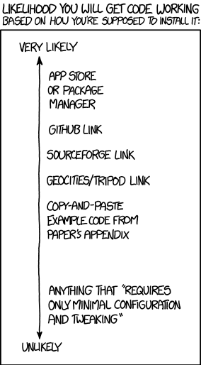
One great thing about using GitHub is that it is a standardised way of obtaining software. When someone asks for your code, you send them the URL of the repo. Assuming that the world is a better place and everyone knows how to use git, you don’t need to do anything else since the repo URL is all they need to get your code. a git clone later and they are in business.
Additionally, you don’t need to worry abut remembering to turn your working directory into a .zip file and uploading it to your website. The code is naturally available for download as part of the standard workflow. No extra thought needed!
In addition to this, some popular computational environments now allow you to install packages directly from GitHub. If, for example, you are following standard good practice for building an R package then a user can install it directly from your GitHub repo from within R using the devtools::install_github() function.
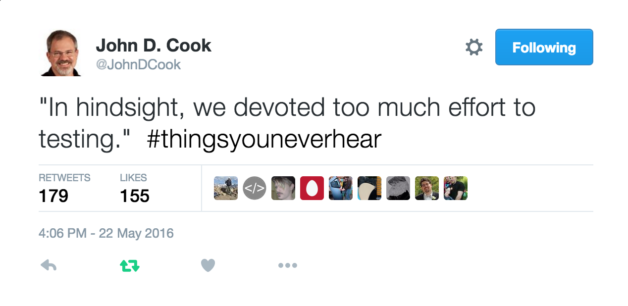
Automatically run all of your tests
You’ve sipped of the KoolAid and you’ve been writing unit tests like a pro. GitHub allows you to link your repo with something called Continuous Integration (CI) that helps maximise the utility of those tests.
Once its all set up the CI service runs every time you, or anyone else, makes a commit to your project. Every time the CI service runs, a virtual machine is created from scratch, your project is installed into it and all of your tests are run with any failures reported.
This gives you increased confidence that everything is OK with your latest version and you can choose to only accept commits that do not break your testing framework.
Collaboration and Community
How git and GitHub can make it easier to collaborate with others on computational projects.
Control exactly who can see your work
‘I don’t want to use GitHub because I want to keep my project private’ is a common reason given to me for not using the service. The ability to create private repositories has been free for some time now (Price plans are available here https://github.com/pricing) and you can have up to 3 collaborators on any of your private repos before you need to start paying. This is probably enough for most small academic projects.
This means that you can control exactly who sees your code. In the early stages it can be just you. At some point you let a couple of trusted collaborators in and when the time is right you can make the repo public so everyone can enjoy and use your work alongside the paper(s) it supports.
Faciliate discussion about your work
Every GitHub repo comes with an Issues section which is effectively a discussion forum for the project. You can use it to keep track of your project To-Do list, bugs, documentation discussions and so on. The issues log can also be integrated with your commit history. This allows you to do things like git commit -m "Improve the foo algorithm according to the discussion in #34" where #34 refers to the Issue discussion where your collaborator pointed out
Allow others to contribute to your work
You have absolute control over external contributions! No one can make any modifications to your project without your explicit say-so.
I start with the above statement because I’ve found that when explaining how easy it is to collaborate on GitHub, the first question is almost always ‘How do I keep control of all of this?’
What happens is that anyone can ‘fork’ your project into their account. That is, they have an independent copy of your work that is clearly linked back to your original. They can happily work away on their copy as much as they like – with no involvement from you. If and when they want to suggest that some of their modifications should go into your original version, they make a ‘Pull Request’.
I emphasised the word ‘Request’ because that’s exactly what it is. You can completely ignore it if you want and your project will remain unchanged. Alternatively you might choose to discuss it with the contributor and make modifications of your own before accepting it. At the other end of the spectrum you might simply say ‘looks cool’ and accept it immediately.
Congratulations, you’ve just found a contributing collaborator.
Reproducible research
How git and GitHub can contribute to improved reproducible research.
Simply making your software available
A paper published without the supporting software and data is (much!) harder to reproduce than one that has both.
Making your software citable
Most modern research cannot be done without some software element. Even if all you did was run a simple statistical test on 20 small samples, your paper has a data and software dependency. Organisations such as the Software Sustainability Institute and the UK Research Software Engineering Association (among many others) have been arguing for many years that such software and data dependencies should be part of the scholarly record alongside the papers that discuss them. That is, they should be archived and referenced with a permanent Digital Object Identifier (DOI).
Once your code is in GitHub, it is straightforward to archive the version that goes with your latest paper and get it its own DOI using services such as Zenodo. Your University may also have its own archival system. For example, The University of Sheffield in the UK has built a system called ORDA which is based on an institutional Figshare instance which allows Sheffield academics to deposit code and data for long term archival.
Which version gave these results?
Anyone who has worked with software long enough knows that simply stating the name of the software you used is often insufficient to ensure that someone else could reproduce your results. To help improve the odds, you should state exactly which version of the software you used and one way to do this is to refer to the git commit hash. Alternatively, you could go one step better and make a GitHub release of the version of your project used for your latest paper, get it a DOI and cite it.
This doesn’t guarentee reproducibility but its a step in the right direction. For extra points, you may consider making the computational environment reproducible too (e.g. all of the dependencies used by your script – Python modules, R packages and so on) using technologies such as Docker, Conda and MRAN but further discussion of these is out of scope for this article.
Building a computational environment based on your repository
Once your project is on GitHub, it is possible to integrate it with many other online services. One such service is mybinder which allows the generation of an executable environment based on the contents of your repository. This makes your code immediately reproducible by anyone, anywhere.
Similar projects are popping up elsewhere such as The Littlest JupyterHub deploy to Azure button which allows you to add a button to your GitHub repo that, when pressed by a user, builds a server in their Azure cloud account complete with your code and a computational environment specified by you along with a JupterHub instance that allows them to run Jupyter notebooks. This allows you to write interactive papers based on your software and data that can be used by anyone.
Complying with funding and journal guidelines
When I started teaching and advocating the use of technologies such as git I used to make a prediction These practices are so obviously good for computational research that they will one day be mandated by journal editors and funding providers. As such, you may as well get ahead of the curve and start using them now before the day comes when your funding is cut off because you don’t. The resulting debate was usually good fun.
My prediction is yet to come true across the board but it is increasingly becoming the case where eyebrows are raised when papers that rely on software are published don’t come with the supporting software and data. Research Software Engineers (RSEs) are increasingly being added to funding review panels and they may be Reviewer 2 for your latest paper submission.
Other uses of git and GitHub for busy academics
It’s not just about code…..
- Build your own websites using GitHub pasges. Every repo can have its own website served directly from GitHub
- Put your presentations on GitHub. I use reveal.js combined with GitHub pages to build and serve my presentations. That way, whenever I turn up at an event to speak I can use whatever computer is plugged into the projector. No more ‘I don’t have the right adaptor’ hell for me.
- Write your next grant proposal. Use Markdown, LaTex or some other git-friendly text format and use git and GitHub to collaboratively write your next grant proposal
The movie below is a visualisation showing how a large H2020 grant proposal called OpenDreamKit was built on GitHub. Can you guess when the deadline was based on the activity?
Further Resources
Further discussions from scientific computing practitioners that discuss using version control as part of a healthy approach to scientific computing
- Good Enough Practices in Scientific Computing –
- Is Your Research Software Correct? – A presentation from Mike Croucher discussing what can go wrong in computational research and what practices can be adopted to do help us do better
- The Turing Way A handbook of good practice in data science brought to you from the Alan Turning Institute
- A guide to reproducible code in ecology and evolution – A handbook from the British Ecological Society that discusses version control as part of general good practice
Learning version control
Convinced? Want to start learning? Let’s begin!
- Git lesson from Software Carpentry – A free, community written tutorial on the basics of git version control
Graphical User Interfaces to git
If you prefer not to use the command line, try these
My stepchildren are pretty good at mathematics for their age and have recently learned about Pythagora’s theorem
$c=\sqrt{a^2+b^2}$
The fact that they have learned about this so early in their mathematical lives is testament to its importance. Pythagoras is everywhere in computational science and it may well be the case that you’ll need to compute the hypotenuse to a triangle some day.
Fortunately for you, this important computation is implemented in every computational environment I can think of!
It’s almost always called hypot so it will be easy to find.
Here it is in action using Python’s numpy module
import numpy as np
a = 3
b = 4
np.hypot(3,4)

5
When I’m out and about giving talks and tutorials about Research Software Engineering, High Performance Computing and so on, I often get the chance to mention the hypot function and it turns out that fewer people know about this routine than you might expect.
Trivial Calculation? Do it Yourself!
Such a trivial calculation, so easy to code up yourself! Here’s a one-line implementation
def mike_hypot(a,b):
    return(np.sqrt(a*a+b*b))
In use it looks fine
mike_hypot(3,4)

5.0
Overflow and Underflow
I could probably work for quite some time before I found that my implementation was flawed in several places. Here’s one
mike_hypot(1e154,1e154)

inf
You would, of course, expect the result to be large but not infinity. Numpy doesn’t have this problem
np.hypot(1e154,1e154)

1.414213562373095e+154
My function also doesn’t do well when things are small.
a = mike_hypot(1e-200,1e-200)

0.0
but again, the more carefully implemented hypot function in numpy does fine.
np.hypot(1e-200,1e-200)

1.414213562373095e-200
Standards Compliance
Next up — standards compliance. It turns out that there is a an official standard for how hypot implementations should behave in certain edge cases. The IEEE-754 standard for floating point arithmetic has something to say about how any implementation of hypot handles NaNs (Not a Number) and inf (Infinity).
It states that any implementation of hypot should behave as follows (Here’s a human readable summary https://www.agner.org/optimize/nan_propagation.pdf)
hypot(nan,inf) = hypot(inf,nan) = inf
numpy behaves well!
np.hypot(np.nan,np.inf)

inf

np.hypot(np.inf,np.nan)

inf
My implementation does not
mike_hypot(np.inf,np.nan)

nan
So in summary, my implementation is
- Wrong for very large numbers
- Wrong for very small numbers
- Not standards compliant
That’s a lot of mistakes for one line of code! Of course, we can do better with a small number of extra lines of code as John D Cook demonstrates in the blog post What’s so hard about finding a hypotenuse?
Hypot implementations in production
Production versions of the hypot function, however, are much more complex than you might imagine. The source code for the implementation used in openlibm (used by Julia for example) was 132 lines long last time I checked. Here’s a screenshot of part of the implementation I saw for prosterity. At the time of writing the code is at https://github.com/JuliaMath/openlibm/blob/master/src/e_hypot.c
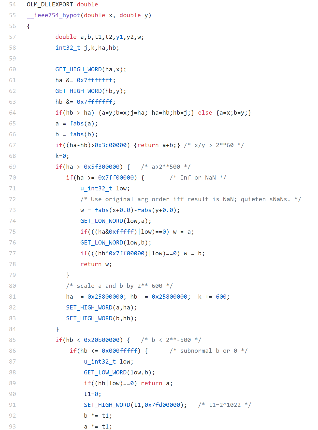
That’s what bullet-proof, bug checked, has been compiled on every platform you can imagine and survived code looks like.
There’s more!
Active Research
When I learned how complex production versions of hypot could be, I shouted out about it on twitter and learned that the story of hypot was far from over!
The implementation of the hypot function is still a matter of active research! See the paper here https://arxiv.org/abs/1904.09481

Is Your Research Software Correct?
Given that such a ‘simple’ computation is so complicated to implement well, consider your own code and ask Is Your Research Software Correct?.
It started with a tweet
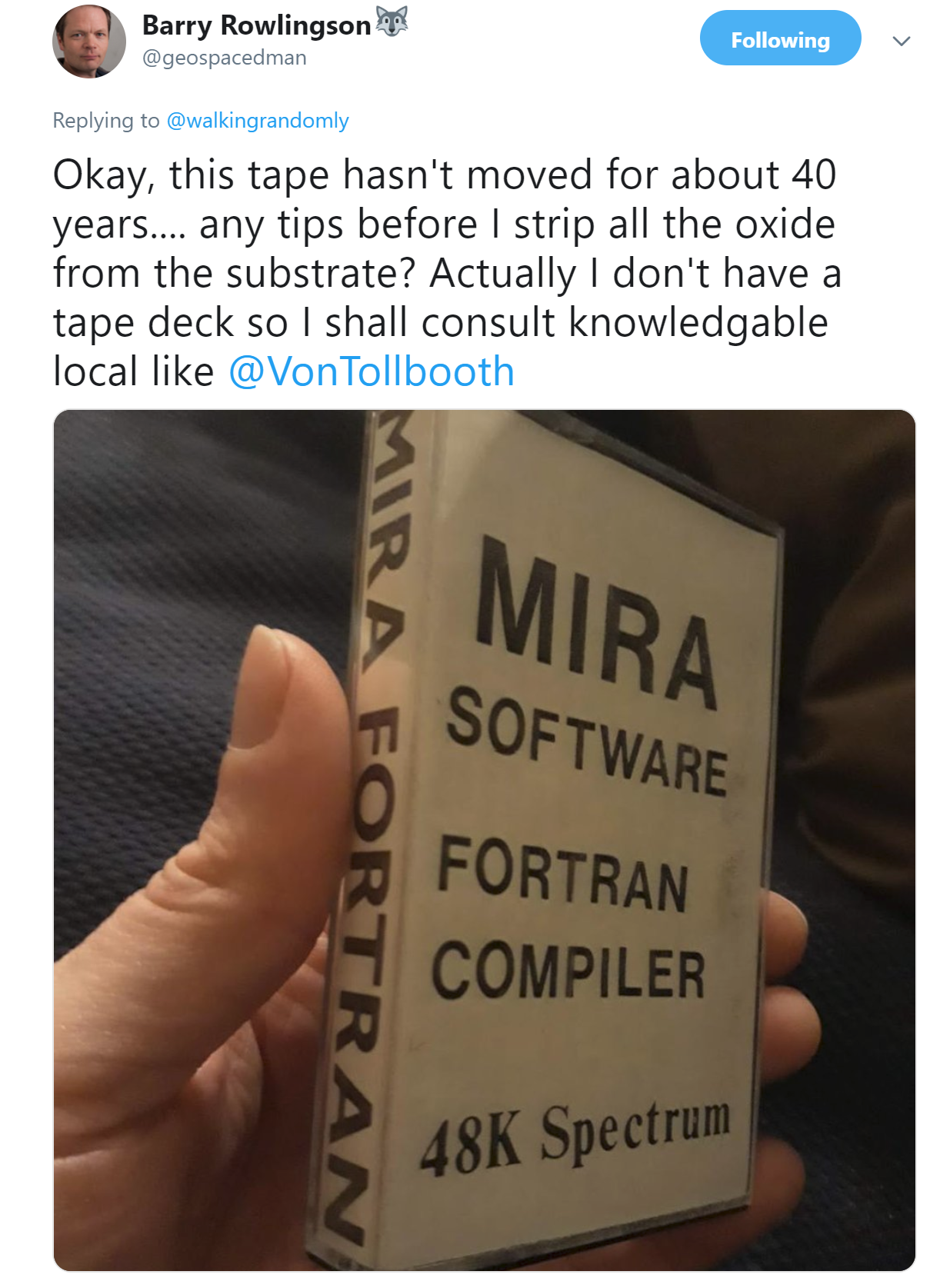
While basking in some geek nostalgia on twitter, I discovered that my first ever microcomputer, the Sinclair Spectrum, once had a Fortran compiler

However, that compiler was seemingly lost to history and was declared Missing in Action on World of Spectrum.

A few of us on Twitter enjoyed reading the 1987 review of this Fortran Compiler but since no one had ever uploaded an image of it to the internet, it seemed that we’d never get the chance to play with it ourselves.
I never thought it would come to this
One of the benefits of 5000+ followers on Twitter is that there’s usually someone who knows something interesting about whatever you happen to tweet about and in this instance, that somebody was my fellow Fellow of the Software Sustainability Institute, Barry Rowlingson. Barry was fairly sure that he’d recently packed a copy of the Mira Fortran Compiler away in his loft and was blissfully unaware of the fact that he was sitting on a missing piece of microcomputing history!
He was right! He did have it in the attic…and members of the community considered it valuable.
As Barry mentioned in his tweet, converting a 40 year old cassette to an archivable .tzx format is a process that could result in permanent failure. The attempt on side 1 of the cassette didn’t work but fortunately, side 2 is where the action was!
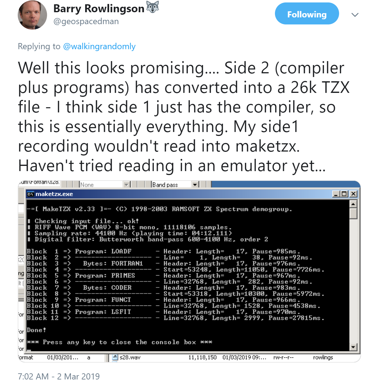
It turns out that everything worked perfectly. On loading it into a Spectrum emulator, Barry could enter and compile Fortran on this platform for the first time in decades! Here is the source code for a program that computes prime numbers

Here it is running

and here we have Barry giving the sales pitch on the advanced functionality of this compiler :)

How to get the compiler
Barry has made the compiler, and scans of the documentation, available at https://gitlab.com/b-rowlingson/mirafortran
I have been an advocate of the Windows Subsytem for Linux ever since it was released (See Bash on Windows: The scripting game just changed) since it allows me to use the best of Linux from my windows laptop. I no longer dual boot on my personal machines and rarely need to use Linux VMs on them either thanks to this technology. I still use full-blown Linux a lot of course but these days it tends to be only on servers and HPC systems.
I recently needed to compile and play with some code that was based on the GNU Scientific Library. Using the Ubuntu 18.04 version of the WSL this is very easy. Install the GSL with
sudo apt-get install libgsl-dev
A simple code that evaluates Dawson’s integral over a range of x values is shown below. Call this dawson.cpp
#include<iostream>
#include<vector>
#include<gsl/gsl_sf.h>

int main(){

double range = 6; // max/min values
int N = 100000; // Number of evaluations
double step = 2 * range / N;
std::vector<double> x(N);
std::vector<double> result(N);

for (int i=0;i<=N;i++){
     x[i] = -range + i*step;
     result[i] = gsl_sf_dawson(x[i]);
}


for (int i=0;i<=N;i++){
	std::cout << x[i] << "," << result[i] << std::endl;
}

return 0;
}
Compile with
g++ -std=c++11 dawson.cpp -o ./dawson -lgsl -lgslcblas -lm
Run it and generate some results
./dawson > results.txt
If we plot results.txt we get
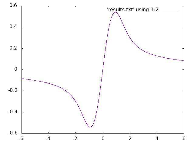
This code is also available on GitHub: https://github.com/mikecroucher/GSL_example
A guest blog-post by Catherine Smith of University of Birmingham
In early 2017 I was in the audience at one of Mike Croucher’s ‘Is your research software correct?’ presentations. One of the first questions posed in the talk is ‘how reproducible is a mouse click?’. The answer, of course, is that it isn’t and therefore research processes should be automated and not involve anyone pressing any buttons. This posed something of a challenge to my own work which is primarily about making buttons for researchers to press (and select, drag and drop etc.) in order to present their data in the appropriate scholarly way. This software, for making electronic editions of texts preserved in multiple sources, assists with the alignment and editing of material. Even so, the editor is always in control and that is the way it should be. The lack of automation means reproducibility is a problem for my software but as Peter Shillingsburg, one of the pioneers of digital editing, says ‘editing is an art not a science’: maybe art can therefore be excused, to an extent, from the constraints of automation and, despite their introduction of human decisions, the buttons may be permitted to stay. Nevertheless I still want to know that my software doing what I think it is doing even if I can’t automate what editors choose to do with it. In the discussion that followed the paper I was talking about the complication of testing my interface-heavy software. Mike agreed that it was a complex situation but concluded by saying “if you go away from here and write one test you will have made the world a better place”.
I did just that. In fact I did very little else for the next three months. What started with one Python unit test has so far led to 65 Python unit tests, 82 Javascript unit tests and 54 functional tests using Selenium. The timing of all of this was perfect in that I had just begun a project to migrate all of our web applications to Django. I had one application partially migrated and so I tested that one and even did some test-driven development on the sections that were not yet complete.
The tests themselves are great to have. This was my first project using Django and I made lots of mistakes in the first application. The tests have been invaluable in ensuring that, as I learned more and made improvements, the older code kept pace with those changes. Now that I have tests for some things I want tests for everything and I have developed a healthy fear of editing code that is not yet tested. There are other advantages as well. When I sat down to write my first test it very quickly became clear that the code I had written was not easily testable. I had to break down the large Django views into smaller chunks of code that could each be unit tested. I now write better structured code because of that time I invested in testing just some of it. I also learned a lot about how to approach migrating all of the remaining applications while writing the detailed tests for every aspect of the first one.T
Django has an integrated test framework based on the python unittest module but with the additional benefit of automatically creating a test database using the models from the project to which test data can be added. It was very straightforward to set up and run (see the Django docs https://docs.djangoproject.com/en/2.1/topics/testing/). I found Javascript unit testing less straight forward. There was not much Javascript in this first application so I used the qunit test framework and sinon.js for mocking. I have never automated the running of these tests and instead just open them in the browser. It’s not ideal but it works for now. I have other applications which are far more Javascript heavy and for those I will need to have automated tests, there are plenty of frameworks around to choose from so I will investigate those when I start writing the tests.
Probably the most important tests I have are the functional tests which are written in Selenium. I had already heard of Selenium, having attended a Test Driven Development workshop several years ago by Harry Percival. I used his book, Test-Driven Development with Python, as a tutorial for all of the Selenium tests and some of the Django and Javascript tests too. Selenium tests are automated browser tests which really do allow you to test what happens when a user presses a button, types text into a text box, selects an item from a list, moves an element by dragging it etc.. The result of every interaction in an interface can be tested with Selenium. The content of each page can also be checked. It is generally not necessary to test static html but I did test the contents of several dynamic pages which loaded different content depending on the permissions granted to a user. Selenium is also integrated within Django using the LiveServerTestCase which means it has access to a copy of the database just like the Django unit tests. Selenium tests can be complex and there are several things to watch out for. Selenium doesn’t automatically wait for a page to load before executing the test statements against it, at every point data is loaded Selenium must be told to wait until a given condition is fulfilled up to a maximum time limit before continuing. I still have tests which occasionally fail because, on that particular run, a page or an ajax call is taking longer to load than I have allowed for. Run it another five times and it may well pass on every one. It is also important to make sure the browser is told to scroll to a point where an element can be seen before the instruction to interact with that element is given. It’s not difficult to do and is more predictable that waiting for a page to load but it still has to be remembered every time.
The functional tests are by far the most complex of all the tests I wrote in my three month testing marathon but they are the most important. I can’t automate the entire creation of a digital edition but with tests I can make sure my interface is presenting the correct data in the right way to the editors and that when they interact with that data everything behaves as it should. I really can say that the buttons and other interactive elements I have tested do exactly what I think they do. Now I just need to test all the rest of the buttons – one test at a time!
Update
A discussion on twitter determined that this was an issue with Locales. The practical upshot is that we can make R act the same way as the others by doing
Sys.setlocale("LC_COLLATE", "C")which may or may not be what you should do!
Original post
While working on a project that involves using multiple languages, I noticed some tests failing in one language and not the other. Further investigation revealed that this was essentially because R's default sort order for strings is different from everyone else's.
I have no idea how to say to R 'Use the sort order that everyone else is using'. Suggestions welcomed.
R 3.3.2
sort(c("#b","-b","-a","#a","a","b"))

[1] "-a" "-b" "#a" "#b" "a" "b"
Python 3.6
sorted({"#b","-b","-a","#a","a","b"})

['#a', '#b', '-a', '-b', 'a', 'b']
MATLAB 2018a
sort([{'#b'},{'-b'},{'-a'},{'#a'},{'a'},{'b'}])

ans =
1×6 cell array
{'#a'} {'#b'} {'-a'} {'-b'} {'a'} {'b'}
C++
int main(){

std::string mystrs[] = {"#b","-b","-a","#a","a","b"};
std::vector<std::string> stringarray(mystrs,mystrs+6);
std::vector<std::string>::iterator it;

std::sort(stringarray.begin(),stringarray.end());

for(it=stringarray.begin(); it!=stringarray.end();++it) {
   std::cout << *it << " ";
}

return 0;
}
Result:
#a #b -a -b a b
I’m working on optimising some R code written by a researcher at University of Sheffield and its very much a war of attrition! There’s no easily optimisable hotspot and there’s no obvious way to leverage parallelism. Progress is being made by steadily identifying places here and there where we can do a little better. 10% here and 20% there can eventually add up to something worth shouting about.
One such micro-optimisation we discovered involved multiplying two matrices together where one of them needed to be transposed. Here’s a minimal example.
#Set random seed for reproducibility
set.seed(3)

# Generate two random n by n matrices
n = 10
a = matrix(runif(n*n,0,1),n,n)
b = matrix(runif(n*n,0,1),n,n)

# Multiply the matrix a by the transpose of b
c = a %*% t(b)
When the speed of linear algebra computations are an issue in R, it makes sense to use a version that is linked to a fast implementation of BLAS and LAPACK and we are already doing that on our HPC system.
Here, I am using version 3.3.3 of Microsoft R Open which links to Intel’s MKL (an implementation of BLAS and LAPACK) on a Windows laptop.
In R, there is another way to do the computation c = a %*% t(b) — we can make use of the tcrossprod function (There is also a crossprod function for when you want to do t(a) %*% b)
c_new = tcrossprod(a,b)
Let’s check for equality
c_new == c
[,1] [,2] [,3] [,4] [,5] [,6] [,7] [,8] [,9] [,10]
[1,] TRUE TRUE TRUE TRUE TRUE TRUE TRUE TRUE TRUE TRUE
[2,] TRUE TRUE TRUE TRUE TRUE TRUE TRUE TRUE TRUE TRUE
[3,] TRUE TRUE TRUE TRUE TRUE TRUE TRUE TRUE TRUE TRUE
[4,] TRUE TRUE TRUE TRUE TRUE TRUE TRUE TRUE TRUE TRUE
[5,] TRUE TRUE TRUE TRUE TRUE TRUE TRUE TRUE TRUE TRUE
[6,] TRUE TRUE TRUE TRUE TRUE TRUE TRUE TRUE TRUE TRUE
[7,] TRUE TRUE TRUE TRUE TRUE TRUE TRUE TRUE TRUE TRUE
[8,] TRUE TRUE TRUE TRUE TRUE TRUE TRUE TRUE TRUE TRUE
[9,] TRUE TRUE TRUE TRUE TRUE TRUE TRUE TRUE TRUE TRUE
[10,] TRUE TRUE TRUE TRUE TRUE TRUE TRUE TRUE TRUE TRUE
Sometimes, when comparing the two methods you may find that some of those entries are FALSE which may worry you!
If that happens, computing the difference between the two results should convince you that all is OK and that the differences are just because of numerical noise. This happens sometimes when dealing with floating point arithmetic (For example, see https://www.walkingrandomly.com/?p=5380).
Let’s time the two methods using the microbenchmark package.
install.packages('microbenchmark')
library(microbenchmark)
We time just the matrix multiplication part of the code above:
microbenchmark(
original = a %*% t(b),
tcrossprod = tcrossprod(a,b)
)


Unit: nanoseconds
expr min lq mean median uq max neval
original 2918 3283 3491.312 3283 3647 18599 1000
tcrossprod 365 730 756.278 730 730 10576 1000
We are only saving microseconds here but that’s more than a factor of 4 speed-up in this small matrix case. If that computation is being performed a lot in a tight loop (and for our real application, it was), it can add up to quite a difference.
As the matrices get bigger, the speed-benefit in percentage terms gets lower but tcrossprod always seems to be the faster method. For example, here are the results for 1000 x 1000 matrices
#Set random seed for reproducibility
set.seed(3)

# Generate two random n by n matrices
n = 1000
a = matrix(runif(n*n,0,1),n,n)
b = matrix(runif(n*n,0,1),n,n)

microbenchmark(
original = a %*% t(b),
tcrossprod = tcrossprod(a,b)
)

Unit: milliseconds
expr min lq mean median uq max neval
original 18.93015 26.65027 31.55521 29.17599 31.90593 71.95318 100
tcrossprod 13.27372 18.76386 24.12531 21.68015 23.71739 61.65373 100
The cost of not using an optimised version of BLAS and LAPACK
While writing this blog post, I accidentally used the CRAN version of R. The recently released version 3.4. Unlike Microsoft R Open, this is not linked to the Intel MKL and so matrix multiplication is rather slower.
For our original 10 x 10 matrix example we have:
library(microbenchmark)
#Set random seed for reproducibility
set.seed(3)

# Generate two random n by n matrices
n = 10
a = matrix(runif(n*n,0,1),n,n)
b = matrix(runif(n*n,0,1),n,n)

microbenchmark(
original = a %*% t(b),
tcrossprod = tcrossprod(a,b)
)

Unit: microseconds
       expr   min    lq    mean median     uq    max neval
   original 3.647 3.648 4.22727  4.012 4.1945 22.611   100
 tcrossprod 1.094 1.459 1.52494  1.459 1.4600  3.282   100
Everything is a little slower as you might expect and the conclusion of this article — tcrossprod(a,b) is faster than a %*% t(b) — seems to still be valid.
However, when we move to 1000 x 1000 matrices, this changes
library(microbenchmark)
#Set random seed for reproducibility
set.seed(3)

# Generate two random n by n matrices
n = 1000
a = matrix(runif(n*n,0,1),n,n)
b = matrix(runif(n*n,0,1),n,n)

microbenchmark(
original = a %*% t(b),
tcrossprod = tcrossprod(a,b)
)

Unit: milliseconds
       expr      min       lq     mean   median       uq       max neval
   original 546.6008 587.1680 634.7154 602.6745 658.2387  957.5995   100
 tcrossprod 560.4784 614.9787 658.3069 634.7664 685.8005 1013.2289   100
As expected, both results are much slower than when using the Intel MKL-lined version of R (~600 milliseconds vs ~31 milliseconds) — nothing new there. More disappointingly, however, is that now tcrossprod is slightly slower than explicitly taking the transpose.
As such, this particular micro-optimisation might not be as effective as we might like for all versions of R.
For a while now, Microsoft have provided a free Jupyter Notebook service on Microsoft Azure. At the moment they provide compute kernels for Python, R and F# providing up to 4Gb of memory per session. Anyone with a Microsoft account can upload their own notebooks, share notebooks with others and start computing or doing data science for free.
They University of Cambridge uses them for teaching, and they’ve also been used by the LIGO people (gravitational waves) for dissemination purposes.
This got me wondering. How much power does Microsoft provide for free within these notebooks? Computing is pretty cheap these days what with the Raspberry Pi and so on but what do you get for nothing? The memory limit is 4GB but how about the computational power?
To find out, I created a simple benchmark notebook that finds out how quickly a computer multiplies matrices together of various sizes.
- The benchmark notebook is here on Azure https://notebooks.azure.com/walkingrandomly/libraries/MatrixMatrix
- and here on GitHub https://github.com/mikecroucher/Jupyter-Matrix-Matrix
Matrix-Matrix multiplication is often used as a benchmark because it’s a common operation in many scientific domains and it has been optimised to within an inch of it’s life. I have lost count of the number of times where my contribution to a researcher’s computational workflow has amounted to little more than ‘don’t multiply matrices together like that, do it like this…it’s much faster’
So how do Azure notebooks perform when doing this important operation? It turns out that they max out at 263 Gigaflops! 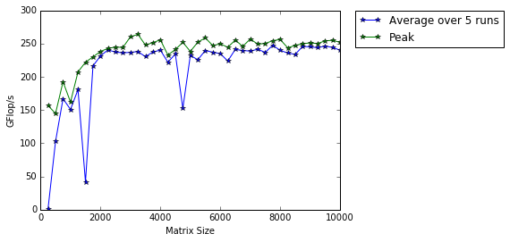
For context, here are some other results:
- A 16 core Intel Xeon E5-2630 v3 node running on Sheffield’s HPC system achieved around 500 Gigaflops.
- My mid-2014 Mabook Pro, with a Haswell Intel CPU hit, hit 169 Gigaflops.
- My Dell XPS9560 laptop, with a Kaby Lake Intel CPU, manages 153 Gigaflops.
As you can see, we are getting quite a lot of compute power for nothing from Azure Notebooks. Of course, one of the limiting factors of the free notebook service is that we are limited to 4GB of RAM but that was more than I had on my own laptops until 2011 and I got along just fine.
Another fun fact is that according to https://www.top500.org/statistics/perfdevel/, 263 Gigaflops would have made it the fastest computer in the world until 1994. It would have stayed in the top 500 supercomputers of the world until June 2003 [1].
Not bad for free!
[1] The top 500 list is compiled using a different benchmark called LINPACK so a direct comparison isn’t strictly valid…I’m using a little poetic license here.
UK to launch 6 major HPC centres
Tomorrow, I’ll be attending the launch event for the UK’s new HPC centres and have been asked to deliver a short talk as part of the program. As someone who paddles in the shallow-end of the HPC pool I find this both flattering and more than a little terrifying. What can little-ole-me say to the national HPC glitterati that might be useful?
This blog post is an attempt at gathering my thoughts together for that talk.
The technology gap in research computing
Broadly speaking, my role in academia is to hang out with researchers, compute providers (cloud and HPC) and software vendors in an attempt to be vaguely useful in the area of research software. I’m a Research Software Engineer with a focus on Long Tail Science: The large number of very small research groups who do a huge amount of modern research.
Time and again, what I see can be summarized in this quote by Greg Wilson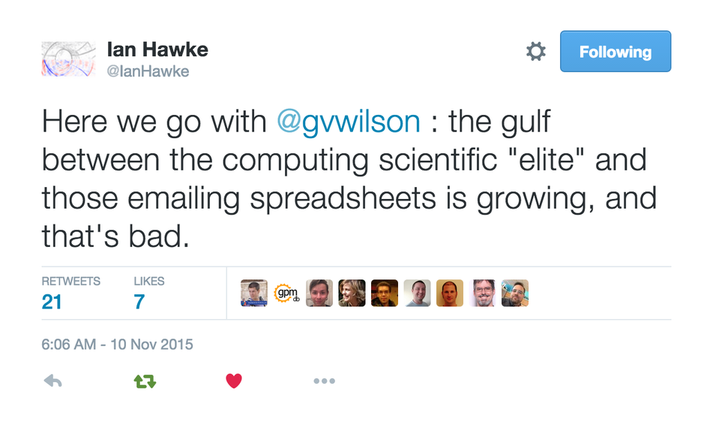
This is very true in the world of High Performance Computing.
Geek Top Gear
I love technology and I love HPC in particular. I love to geek out on Flops, Ghz, SIMD instructions, GPUs, FPGAs…..all that stuff. I help support The University of Sheffield’s local HPC service and worked in Research IT at The University of Manchester for around a decade before moving to Sheffield.
I’ve given and seen many a HPC-related talk in my time and have certainly been guilty of delivering what I now refer to as the ‘Geek Top Gear’ speech. For maximum effect, you need to do it in a Jeremy Clarkson voice and, if you’re feeling really macho, kiss your bicep at the point where you tell the audience how many Petaflops your system can do in Linpack.
*Begin Jeremy Clarkson Impression*
Our new HPC system has got 100,000 of the latest Intel Kaby Lake cores...which is a lot!
Usually running at 2.6Ghz, these cores can turbo-boost to 3.2Ghz for those moments when we need that extra boost of power. Obviously, being Kaby Lake, these cores have all the instruction extensions you’d expect with AVX2, FMA, SSE, ABM and many many other TLAs for all your SIMD needs. Of course every HPC system needs accelerators…..and we have the best of them: Xeon Phis with 68 cores each and NVIDIA GPUs with thousands of tiny little cores will handle every massively parallel job you can throw at them….Easily. We connect these many many cores together with high-speed interconnect fashioned from threads of pure unicorn hair and cool the whole thing with the tears of virigin nerds.
YEEEEEES! Our new HPC system is the best one since the last one and, achieving over a Gajillion Petaflops in the Linpack test (kiss bicep), it will change your life forever.

Any questions?
Audience member 1: What’s a core?
Audience member 2: Why does it run my R script slower than my laptop?
Audience member 3: Do you have Excel installed on it?
There is a huge gap between what many HPC providers like to focus on and what the typical long-tail researcher wants or needs. I propose that the best bridge for this gap is the Research Software Engineer (RSE).
Research Software Engineer as Alpine guide
In my fellowship proposal, I compared the role of a Research Software Engineer to that of an alpine guide:
Technological development in software is more like a cliff-face than a ladder – there are many routes to the top, to a solution. Further, the cliff face is dynamic – constantly and quickly changing as new technologies emerge and decline. Determining which technologies to deploy and how best to deploy them is in itself a specialist domain, with many features of traditional research.
Researchers need empowerment and training to give them confidence with the available equipment and the challenges they face. This role, akin to that of an Alpine guide, involves support, guidance, and load carrying. When optimally performed it results in a researcher who knows what challenges they can attack alone, and where they need appropriate support. Guides can help decide whether to exploit well-trodden paths or explore new possibilities as they navigate through this dynamic environment.
At Sheffield, we have built a pool of these Research Software Engineers to provide exactly this kind of support and it’s working extremely well so far. Not only are we helping individual research groups but we are also using our experiences in the field to help shape the University HPC environment in collaboration with the IT department.
Supercomputing: Irrelevant to many?
“Never bring an anecdote to a data-fight” so the saying goes and all I have from my own experiences are a bucket load of anecdotes, case studies and cursory log-mining experiments that indicate that even those who DO use HPC are not doing so effectively. Fortunately, others have stepped up to the plate and we have survey and interview data on how researchers are using compute resources.
How Do Scientists Develop and Use Scientific Software? is a report on a 2009 survey of 1972 researchers from around the world. They found that “79.9% of the scientists never use scientific software on a supercomputer”
When I first learned of this number, I found it faintly depressing. This technology that I love so much and for which University IT departments dedicate special days to seems to be pretty much irrelevant to the majority of researchers. Could it be that even in an era of big data, machine learning and research software engineering that most people only need a laptop?
Only ever needing a laptop certainly doesn’t fit with what I’ve seen while working in the trenches. Almost every researcher I’ve met who does computational research wishes it was faster or that they had more memory to allow them to do larger problems. Speed is the easiest thing to sell to researchers in the world of RSE. They come for faster execution and leave with a side-order of version control, testing and documentation. A combination of software development and migration to even a small HPC system can easily result in 100x or even 1000x speed-ups for many researchers.
In my experience, it’s not that researchers don’t need HPC, it’s that the jump from their laptop-based workflow to one that makes good use of a HPC system is too large for them to bridge without a little help. Providing that help can result in some great partnerships such as the recent one between the Sheffield RSE group and the Sheffield Faculty of Arts and Humanities.

Want to know how that partnership started? I compiled an experimental R/Rcpp package that they were struggling with and then took them for coffee and said ‘That code took a while to run. Here’s how we can make it go faster….Now…what exactly are you doing because it looks cool?’ Fast forward a year or so and we are on the cusp of starting a great new project that will include traditional HPC and cloud computing as part of their R-based workflow.
My experiences seem to be reflected in the data. In their 2011 article, A Survey of the Practice of Computational Science, Prabhu et al interviewed 114 randomly selected researchers from Princeton University. Princeton have a very strong, well supported HPC centre which provides both resources and the expertise to use them. Even at such a well equipped institution, the authors write that ‘Despite enormous wait times, many scientists run their programs only on desktops’ although they did report much higher HPC usage compared to the Hanny et al survey.
Other salient quotes from the Prabhu interviews include
“only 18% of researchers who optimize code leveraged profiling tools to inform their optimization plans”
“only 7% of researchers leveraged any form of thread based shared memory CPU parallelism”
“Only 11% of researchers utilized loop based parallelism”
“Currently, many researchers fit their scientific models to only a subset of available parameters for faster program runs.”
“Across disciplines, an order of magnitude performance improvement was cited as a requirement for significant changes in research quality”
HPC: There’s plenty of room at the bottom
Potential users of HPC look different to those of 20 years ago. The popularity explosion of languages such as MATLAB, Python and R have democratized programming and the world is awash with inefficient research software. Most of the time, this lack of efficiency is not a problem (see ‘In defense of inefficient scientific code‘) but if a researcher needs to scale up what they are doing, it can become limiting. Researchers might wait for days for the results to come in and limit the scope of their investigations to fit the hardware they have access to — their laptop usually.
The paper of Prabu et al said that an order of magnitude (10x) speed up was cited by researchers as a requirement for significant changes in research quality. For an experienced Research Software Engineer with access to cloud or HPC facilities, a 10x speed-up is usually pretty easy to achieve for this new audience. 100x or even 1000x can be achieved fairly frequently if you employ multiple hardware and software techniques. Compared to squeezing out a few percent more performance from HPC-centric code such as LAPACK or CASTEP, it’s not even all that difficult. I recently sped up one researcher’s MATLAB code by a factor of 800x in a couple of days and I’m a fairly middling developer if I’m brutally honest.
The whole point of High Performance Computing is to accelerate science and right now there is more computational science around than there has ever been before. Furthermore, it’s easier than ever to accelerate! There’s plenty of room at the bottom.
Closing the computational gap with people, training and compute power
The UK’s 6 new HPC centers represent the cutting edge of hardware technology. They provide a crucial component of our national hardware infrastructure, will contribute to research in HPC itself and will doubtless be of huge benefit to computational science. Furthermore, all of the funded proposals include significant engagement with the national Research Software Engineering community – the vital bridge between many researchers and HPC.
Co-development of research software with effort from both RSEs and researchers can be an extremely powerful model. Combine this with further collaboration between RSEs and compute providers and we have an environment that I think is both very exciting and capable of helping to close the rich/poor compute divide.
As an RSE who works with both researchers and University-level HPC providers, I ask for 3 things to be considered by these new regional centres.
- Enjoy your new compute-ferraris. I look forward to seeing how hard you can push them.
- You will be learning new good practice in how to provide HPC services. Disseminate this to those of us running smaller services.
- There’s plenty of room at the bottom! Help us to support the new wave of computational researchers.
Thanks to languages such as MATLAB, Python and R, general purpose programming has been fully democratized. I look forward to working with these new centres to help democratize high performance computing.