Archive for the ‘Wolfram Demonstrations’ Category
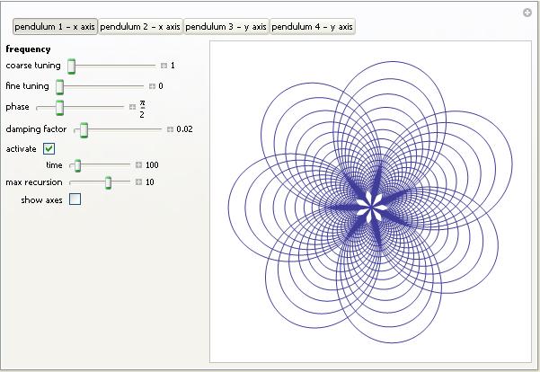
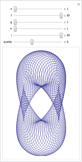
Over at Playing with Mathematica, Sol Lederman has been looking at pretty parametric and polar plots. One of them really stood out for me, the one that Sol called ‘Slinky Thing’ which could be generated with the following Mathematica command.
ParametricPlot[{Cos[t] - Cos[80 t] Sin[t], 2 Sin[t] - Sin[80 t]}, {t, 0, 8}]
Out of curiosity I parametrised some of the terms and wrapped the whole thing in a Manipulate to see what I could see. I added 5 controllable parameters by turning Sol’s equations into
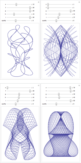
{Cos[e t] - Cos[f t] Sin[g t], 2 Sin[h t] - Sin[i t]}, {t, 0, 8}
Each parameter has its own slider (below). If you have Mathematica 8, or the free cdf player, installed then the image below will turn into an interactive applet which you can use to explore the parameter space of these equations.
Here are four of my favourites. If you come up with one that you particularly like then feel free to let me know what the parameters are in the comments.
I have been a huge fan of the Wolfram Demonstrations project ever since it was launched and have even contributed a few simple demonstrations myself. The project contains thousands of fully interactive mathematical demonstrations that anyone can play with using Wolfram’s free player software and it’s just got a whole lot better.
Now, you can interact with these demonstrations right from the web-browser!
Take the image below, for example. If you don’t have a copy of Wolfram’s new cdf (computable document format) player installed then you’ll just see a static image. Install the player (or Mathematica 8 and the browser-plug in), however, and this image will turn into a fully interactive example.
At the moment the browser plug-in only works on Windows and Macintosh but hopefully a Linux version will be on the way soon. Stay tuned to WalkingRandomly for in-depth tutorials on how to go from Mathematica code to fully interactive mathematics in your browser. The results can be incorporated into the Wolfram Demonstrations project or embedded in your own website like I’ve done here.
Links
- Simulating Harmonographs – Wondering what the above demo is based on? Find out here.
- Wolfram Demonstrations Project – Freshly re-designed as of 8th March 2011
- CDF Player – Download Wolfram’s new (and free) Computable Document Format (CDF) player
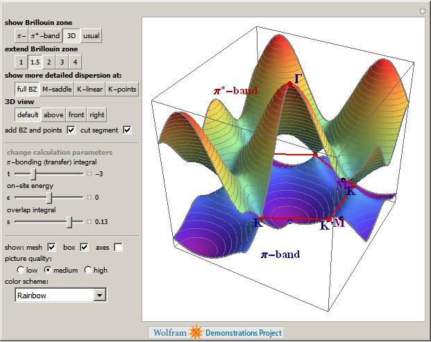
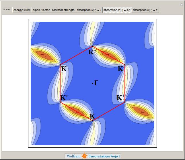
I work at The University of Manchester in the UK and, as some of you may have heard, two of our Professors recently won the Nobel Prize in physics for their discovery of graphene. Naturally, I wanted to learn more about graphene and, as a fan of Mathematica, I turned to the Wolfram Demonstrations Project to see what I could see. Click on the images to go to the relevant demonstration.
Back when I used to do physics research myself, I was interested in band structure and it turns out that there is a great demonstration from Vladimir Gavryushin that will help you learn all about the band structure of graphene using the tight binding approximation.
The electronic band structure of a material is important because it helps us to understand (and maybe even engineer) its electronic and optical properties and if you want to know more about its optical properties then the next demonstration from Jessica Alfonsi is for you.
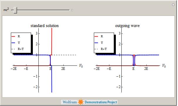
Another professor at Manchester, Niels Walet, produced the next demonstration which asks “Is there a Klein Paradox in Graphene?”
Finally, Graphene can be rolled up to make Carbon Nanotubes as demonstrated by Sándor Kabai.
This is just a taster of the Graphene related demonstrations available at The Wolfram Demonstrations project (There are 11 at the time of writing) and I have no doubt that there will be more in the future. Many of them are exceptionally well written and they include lists of references, full source code and, best of all, they can be run for free using the Mathematica Player.
Don’t just read about cutting-edge research, get in there and interact with it!
Regular readers of Walking Randomly will know that I am a big fan of the Manipulate function in Mathematica. Manipulate allows you to easily create interactive mathematical demonstrations for teaching, research or just plain fun and is the basis of the incredibly popular Wolfram Demonstrations Project.
Sage, probably the best open source mathematics software available right now, has a similar function called interact and I have been playing with it a bit recently (see here and here) along with some other math bloggers. The Sage team have done a fantastic job with the interact function but it is missing a major piece of functionality in my humble opinion – a Locator control.
In Mathematica the default control for Manipulate is a slider:
Manipulate[Plot[Sin[n x], {x, -Pi, Pi}], {n, 1, 10}]

The slider is also the default control for Sage’s interact:
@interact
def _(n=(1,10)):
    plt=plot(sin(n*x),(x,-pi,pi))
    show(plt)

Both systems allow the user to use other controls such as text boxes, checkboxes and dropdown menus but Mathematica has a control called a Locator that Sage is missing. Locator controls allow you to directly interact with a plot or graphic. For example, the following Mathematica code (taken from its help system) draws a polygon and allows the user to click and drag the control points to change its shape.
Manipulate[Graphics[Polygon[pts], PlotRange -> 1],
 {{pts, {{0, 0}, {.5, 0}, {0, .5}}}, Locator}]

The Locator control has several useful options that allow you to customise your demonstration even further. For example, perhaps you want to allow the user to move the vertices of the polygon but you don’t want them to be able to actually see the control points. No problem, just add Appearance -> None to your code and you’ll get what you want.
Manipulate[Graphics[Polygon[pts], PlotRange -> 1],
 {{pts, {{0, 0}, {.5, 0}, {0, .5}}}, Locator, Appearance -> None}]
Another useful option is LocatorAutoCreate -> True which allows the user to create extra control points by holding down CTRL and ALT (or just ALT – it depends on your system it seems) as they click in the active area.
Manipulate[Graphics[Polygon[pts], PlotRange -> 1],
 {{pts, {{0, 0}, {.5, 0}, {0, .5}}}, Locator,
  LocatorAutoCreate -> True}]
When you add all of this functionality together you can do some very cool stuff with just a few lines of code. Theodore Gray’s curve fitting code on the Wolfram Demonstrations project is a perfect example.
All of these features are demonstrated in the video below
So, onto the bounty hunt. I am offering 25 pounds worth (about 40 American Dollars) of books from Amazon to anyone who writes the code to implement a Locator control for Sage’s interact function. To get the prize your code must fulfil the following spec
- Your code must be accepted into the Sage codebase and become part of the standard install. This should ensure that it is of reasonable quality.
- There should be an option like Mathematica’s LocatorAutoCreate -> True to allow the user to create new locator points interactively by Alt-clicking (or via some other suitable method).
- There should be an option to alter the appearance of the Locator control (e.g. equivalent to Mathematica’s Appearance -> x option). As a minimum you should be able to do something like Appearance->None
- You should provide demonstration code that implements everything shown in the video above.
- I have to be happy with it!
And the details of the prize:
- I only have one prize – 25 pounds worth of books (about 40 American dollars) from Amazon. If more than one person claims it then the prize will be split.
- The 25 pounds includes whatever it will cost for postage and packing.
- I won’t send you the voucher – I will send you the books of your choice as a ‘gift’. This will mean that you’ll have to send me your postal address. Don’t enter if this bothers you for some reason.
- I expect you to be sensible regarding the exact value of the prize. So if your books come to 24.50 then we’ll call it even. Similarly if they come to 25.50 then I won’t argue.
- I am not doing this on behalf of any organisation. It’s my personal money.
- My decision is final and I can withdraw this prize offer at any time without explanation. I hope you realise that I am just covering my back by saying this – I have every intention of giving the prize but whenever money is involved one always worries about the possibility of being ripped off.
Good luck!
Update (29th December 2009): The bounty hunt has only been going for a few days and the bounty has already doubled to 50 pounds which is around 80 American dollars. Thanks to David Jones for his generosity.
Earlier today I was chatting to a lecturer over coffee about various mathematical packages that he might use for an upcoming Masters course (note – offer me food or drink and I’m happy to talk about pretty much anything). He was mainly interested in Mathematica and so we spent most of our time discussing that but it is part of my job to make sure that he considers all of the alternatives – both commercial and open source. The course he was planning on running (which I’ll keep to myself out of respect for his confidentiality) was definitely a good fit for Mathematica but I felt that SAGE might suite him nicely as well.
“Does it have nice, interactive functionality like Mathematica’s Manipulate function?” he asked
Oh yes! Here is a toy example that I coded up in about the same amount of time that it took to write the introductory paragraph above (but hopefully it has no mistakes). With just a bit of effort pretty much anyone can make fully interactive mathematical demonstrations using completely free software. For more examples of SAGE’s interactive functionality check out their wiki.

Here’s the code:
def ftermSquare(n):
 return(1/n*sin(n*x*pi/3))

def ftermSawtooth(n):
 return(1/n*sin(n*x*pi/3))

def ftermParabola(n):
 return((-1)^n/n^2 * cos(n*x))

def fseriesSquare(n):
 return(4/pi*sum(ftermSquare(i) for i in range (1,2*n,2)))

def fseriesSawtooth(n):
 return(1/2-1/pi*sum(ftermSawtooth(i) for i in range (1,n)))

def fseriesParabola(n):
 return(pi^2/3 + 4*sum(ftermParabola(i) for i in range(1,n)))

@interact
def plotFourier(n=slider(1, 30,1,10,'Number of terms')
,plotpoints=('Value of plot_points',[100,500,1000]),Function=['Saw Tooth','Square Wave','Periodic Parabola']):
    if Function=='Saw Tooth':
     show(plot(fseriesSawtooth(n),x,-6,6,plot_points=plotpoints))
    if Function=='Square Wave':
     show(plot(fseriesSquare(n),x,-6,6,plot_points=plotpoints))
    if Function=='Periodic Parabola':
     show(plot(fseriesParabola(n),x,-6,6,plot_points=plotpoints))
Take a wheel of radius 1 and set it rotating about its axis with a frequency of 1 turn per second. Attach a second wheel, of radius 1/2, to the circumference of the first and set this second wheel rotating about its axis at a frequency of 7 turns per second. Finally, attach a third wheel to the circumference of the second and set this wheel to rotate about it’s axis at a frequency of 17 turns per second.
Now, consider a point on the circumference of the third wheel. What pattern will it trace out as the three wheels rotate? Click on the video below to find out.
I first came across this idea in a Wolfram demonstration by Daniel de Souza Carvalho. Daniel’s demonstration focused on the fact that you could write down the equations of these curves in two different ways. If the wheels are rotating with frequencies a, b and c respectively then you can either describe the corresponding curve with a pair of parametric equations as follows:
![]()
![]()
or as a complex valued equation:
![]()
This was a nice demonstration but I wanted to see what sort of patterns I could get by changing the frequencies of the wheels. So, I downloaded Daniel’s demonstration, added some sliders and tick boxes and then uploaded the result. Wolfram Research cleaned up my code a bit and the result was published as the Wolfram Demonstration Wheels on Wheels on Wheels.
It turns out that you can get a LOT of different patterns out of this system as you can see below.

These systems were considered in the paper “Wheels on Wheels on Wheels—Surprising Symmetry,” Mathematics Magazine 69(3), 1996 pp. 185–189 by F. A. Farris. In this paper, Farris showed that the resulting curve exhibits m-fold symmetry if the three frequencies are congruent (mod m).
Can you think of any interesting variations to this system?
Update (6th July 2009): Taki has written another version of this demonstration which includes an animation of the wheels and also looked at an example with four wheels over at his blog, Mesh Mess.
I first came across Albrecht Dürer, an artist from the 15th and 16th centuries, while looking into pentaflakes a little while back. In the comments section of the pentaflake post someone pointed me to a wonderful picture of a Rhino drawn by Dürer.

What makes this picture particularly amazing to me is that Dürer had never even seen a Rhino when he produced it. Well, thanks to the Wolfram Demonstrations project, Dürer has made another appearance in my consciousness. It turns out that he laid out a recipe for producing a heptagon using nothing more than a straight-edge and a compass and Ralf Schaper has brought this bang up to date by showing all of the steps in a Wolfram Demonstration.
I wonder what other mathematics Dürer had a hand in?
Here in the UK we have had more snow than we have seen in over 20 years and as a country we are struggling with it to say the least. I have friends in places such as Finland who think that all this is rather funny…it takes nothing more than a bit of snow to bring the UK to its knees.
Anyway…all this talk of snow reminds me of a Wolfram Demonstration I authored around Christmas time called n-flakes. It started off while I was playing with the so called pentaflake which was first described by someone called Albrecht Dürer (according to Wolfram’s Mathworld). To make a pentaflake you first start of with a pentagon like this one.

Your next step is to get five more identical pentagons and place each one around the edges of the first as follows

The final result is the first iteration of the pentaflake design. Take a closer look at it….notice how the outline of the pentaflake is essentially a pentagon with some gaps in it?

Lets see what happens if we take this ‘gappy’ pentagon and arrange 5 identical gappy pentagons around it – just like we did in the first iteration.

The end result is a more interesting looking gappy pentagon. If we keep going in this manner then you eventually end up with something like this
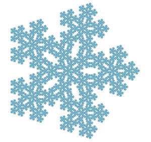
Which is very pretty I think. Anyway, over at Mathworld, Eric Weisstein had written some Mathematica code to produce not only this variation of a pentaflake but also another one which was created by putting pentagons at the corners of the first one rather than the sides. Also, rather than using identical pentagons, this second variation used scaled pentagons for each iteration. The end result is shown below.

Looking at Eric’s code I discovered that it would be a trivial matter to wrap this up in a Manipulate function and produce an interactive version. This took about 30 seconds – the quickest Wolfram demonstration I had ever written. After submitting it (with due credit being given to Eric) I got an email back from the Wolfram Demonstration team saying ‘Why stop at just pentagons? Could you generalise it a bit before we publish it?’
So I did and the result was named N-flakes which is available for download on the Wolfram Demonstrations site. Along with pentaflakes, you can also play with hexaflakes, quadraflakes and triflakes. One or two of these usually go by slightly different names – kudos for anyone who finds them.

The Wolfram Demonstrations project has been updated to take advantage of the new features of version 7 of Mathematica and Jeff Bryant has written a great post about it on the Wolfram Research Blog. As you might expect, Wolfram have also upgraded their free Mathematica player which allows you to run all of their demonstrations without a Mathematica license.
Some of the new demonstrations are very pretty! I particularly like their new vector field plotting routines as shown in the demonstration below which calculates the electric field pattern formed by three point charges.
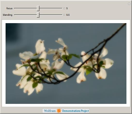
The new image processing routines that Wolfram have added to Mathematica allow for the easy production of some very beautiful demonstrations. Here is one by Peter Overmann that simulates a photographic technique called the Orton Effect.
The Wolfam Demonstrations project has just topped 4000 submissions! I make no secret of the fact that I love the Wolfram Demonstrations project and barely a day goes by where I don’t mention it to someone. It’s got so bad that I am sometimes accused of being a secret employee of Wolfram Research (I’m not – just for the record – but they are free to make me an offer.) If you are new around here then here is a quick summary of why I like it so much.
- Over 4000 demonstrations covering a very wide range of disciplines.
- Every demonstration is fully interactive and can be used for free via the Mathematica player.
- Full Mathematica source code for every demonstration is easily available. So, if you have a full copy of Mathematica then you can modify them for your own purposes.
- Everyone who has a fully licensed copy of Mathematica can contribute. This is a true community project.
- The guys and gals at Wolfram vet each and every one of the submissions to ensure that they meet various guidelines. If you are an author of a demonstration then they give advice on how you might improve your submission. Sometimes they even supply code that you might not have been able to come up with yourself.
In my opinion, the project really is all things to all people. For example, if you are a teacher then you might use some of the demonstrations to spice up your courses at no cost. Remember – you can download the free Mathematica Player and use all of the demonstrations fully interactively. There is no need to buy a Mathematica license! I often hear maths educators say “The only way to learn mathematics is to do mathematics.” and they are absolutely right! The Wolfram Demonstrations project gives you and your students another way to ‘do math’. Have you just taught some Fourier analysis? Well then, you might be interested in some examples of Fourier Series or maybe you would like to discuss (and demonstrate) Fourier sound synthesis. You might decide to demonstrate how the Fourier Transform can be used for image compression or maybe show the problems that Fourier series have with discontinuites.
If none of the demonstrations do quite what you want then download the source code and modify them. If you don’t have a full copy of Mathematica or the required programming skills then send a request to Wolfram and they may be able to help. Alternatively ask me – I’ll help whenever I can and have done so in the past both for readers of this blog and for teachers and researchers at my place of work (The University of Manchester).
If you are learning how to use Mathematica and prefer to learn from examples then the project is perfect. 4000+ real-world examples right at your fingertips. For free! I have used Mathematica for over 8 years now and yet I constantly come across new techniques and ideas by reading the source code of other author’s submissions.
Perhaps you are not a programmer or a teacher and you just like fiddling around with Mathematics? Again, the Wolfram Demonstrations project is for you. You might choose to play a relaxing game of Tangrams or challenge your brain with Sudoku. Alternatively you be interested in some of the mathematics behind prime numbers or perhaps you want to play around with polygonal numbers?
So, what would you like to see? Although there are over 4000 different demonstrations so far, there is still a lot of stuff left to cover. What is your personal wish list for the Demonstrations project? If you ask you might get ;)
If you enjoyed this article, feel free to click here to subscribe to my RSS Feed.

