
Archive for the ‘python’ Category
My stepchildren are pretty good at mathematics for their age and have recently learned about Pythagora’s theorem
$c=\sqrt{a^2+b^2}$
The fact that they have learned about this so early in their mathematical lives is testament to its importance. Pythagoras is everywhere in computational science and it may well be the case that you’ll need to compute the hypotenuse to a triangle some day.
Fortunately for you, this important computation is implemented in every computational environment I can think of!
It’s almost always called hypot so it will be easy to find.
Here it is in action using Python’s numpy module
import numpy as np
a = 3
b = 4
np.hypot(3,4)

5
When I’m out and about giving talks and tutorials about Research Software Engineering, High Performance Computing and so on, I often get the chance to mention the hypot function and it turns out that fewer people know about this routine than you might expect.
Trivial Calculation? Do it Yourself!
Such a trivial calculation, so easy to code up yourself! Here’s a one-line implementation
def mike_hypot(a,b):
    return(np.sqrt(a*a+b*b))
In use it looks fine
mike_hypot(3,4)

5.0
Overflow and Underflow
I could probably work for quite some time before I found that my implementation was flawed in several places. Here’s one
mike_hypot(1e154,1e154)

inf
You would, of course, expect the result to be large but not infinity. Numpy doesn’t have this problem
np.hypot(1e154,1e154)

1.414213562373095e+154
My function also doesn’t do well when things are small.
a = mike_hypot(1e-200,1e-200)

0.0
but again, the more carefully implemented hypot function in numpy does fine.
np.hypot(1e-200,1e-200)

1.414213562373095e-200
Standards Compliance
Next up — standards compliance. It turns out that there is a an official standard for how hypot implementations should behave in certain edge cases. The IEEE-754 standard for floating point arithmetic has something to say about how any implementation of hypot handles NaNs (Not a Number) and inf (Infinity).
It states that any implementation of hypot should behave as follows (Here’s a human readable summary https://www.agner.org/optimize/nan_propagation.pdf)
hypot(nan,inf) = hypot(inf,nan) = inf
numpy behaves well!
np.hypot(np.nan,np.inf)

inf

np.hypot(np.inf,np.nan)

inf
My implementation does not
mike_hypot(np.inf,np.nan)

nan
So in summary, my implementation is
- Wrong for very large numbers
- Wrong for very small numbers
- Not standards compliant
That’s a lot of mistakes for one line of code! Of course, we can do better with a small number of extra lines of code as John D Cook demonstrates in the blog post What’s so hard about finding a hypotenuse?
Hypot implementations in production
Production versions of the hypot function, however, are much more complex than you might imagine. The source code for the implementation used in openlibm (used by Julia for example) was 132 lines long last time I checked. Here’s a screenshot of part of the implementation I saw for prosterity. At the time of writing the code is at https://github.com/JuliaMath/openlibm/blob/master/src/e_hypot.c
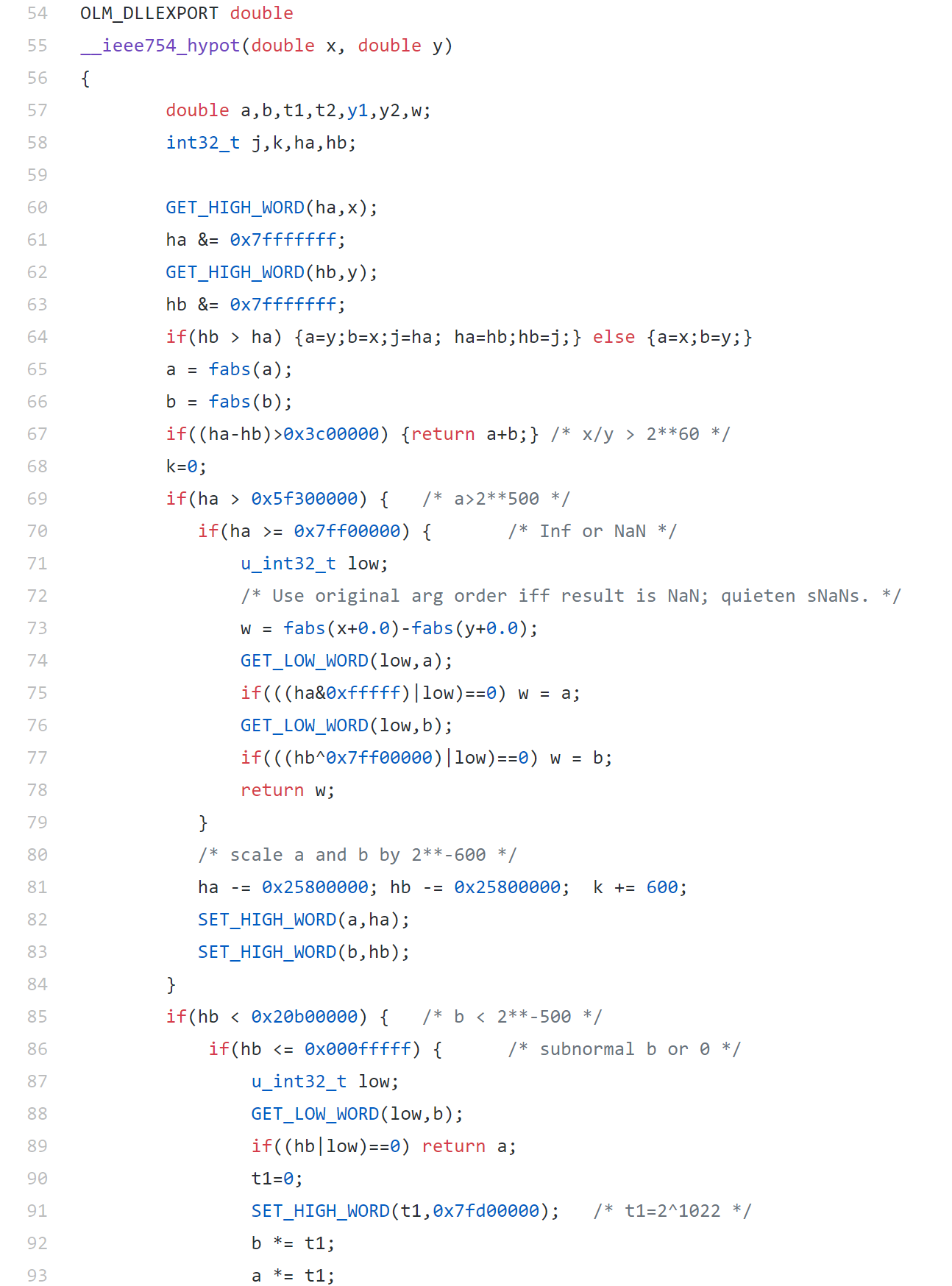
That’s what bullet-proof, bug checked, has been compiled on every platform you can imagine and survived code looks like.
There’s more!
Active Research
When I learned how complex production versions of hypot could be, I shouted out about it on twitter and learned that the story of hypot was far from over!
The implementation of the hypot function is still a matter of active research! See the paper here https://arxiv.org/abs/1904.09481

Is Your Research Software Correct?
Given that such a ‘simple’ computation is so complicated to implement well, consider your own code and ask Is Your Research Software Correct?.
In many introductions to numpy, one gets taught about np.ones, np.zeros and np.empty. The accepted wisdom is that np.empty will be faster than np.ones because it doesn’t have to waste time doing all that initialisation. A quick test in a Jupyter notebook shows that this seems to be true!
import numpy as np

N = 200
zero_time = %timeit -o some_zeros = np.zeros((N,N))
empty_time = %timeit -o empty_matrix = np.empty((N,N))
print('np.empty is {0} times faster than np.zeros'.format(zero_time.average/empty_time.average))


8.34 µs ± 202 ns per loop (mean ± std. dev. of 7 runs, 100000 loops each)
436 ns ± 10.6 ns per loop (mean ± std. dev. of 7 runs, 1000000 loops each)
np.empty is 19.140587654682545 times faster than np.zeros
20 times faster may well be useful in production when using really big matrices. Might even be worth the risk of dealing with uninitialised variables even though they are scary!
However…..on my machine (Windows 10, Microsoft Surface Book 2 with 16Gb RAM), we see the following behaviour with a larger matrix size (1000 x 1000).
import numpy as np

N = 1000
zero_time = %timeit -o some_zeros = np.zeros((N,N))
empty_time = %timeit -o empty_matrix = np.empty((N,N))
print('np.empty is {0} times faster than np.zeros'.format(zero_time.average/empty_time.average))


113 µs ± 2.97 µs per loop (mean ± std. dev. of 7 runs, 10000 loops each)
112 µs ± 1.01 µs per loop (mean ± std. dev. of 7 runs, 10000 loops each)
np.empty is 1.0094651980894993 times faster than np.zeros
The speed-up has vanished! A subsequent discussion on twitter suggests that this is probably because the operating system is zeroing all of the memory for security reasons when using numpy.empty on large arrays.
What is Second Order Cone Programming (SOCP)?
Second Order Cone Programming (SOCP) problems are a type of optimisation problem that have applications in many areas of science, finance and engineering. A summary of the type of problems that can make use of SOCP, including things as diverse as designing antenna arrays, finite impulse response (FIR) filters and structural equilibrium problems can be found in the paper ‘Applications of Second Order Cone Programming’ by Lobo et al. There are also a couple of examples of using SOCP for portfolio optimisation in the GitHub repository of the Numerical Algorithms Group (NAG).
A large scale SOCP solver was one of the highlights of the Mark 27 release of the NAG library (See here for a poster about its performance). Those who have used the NAG library for years will expect this solver to have interfaces in Fortran and C and, of course, they are there. In addition to this is the fact that Mark 27 of the NAG Library for Python was released at the same time as the Fortran and C interfaces which reflects the importance of Python in today’s numerical computing landscape.
Here’s a quick demo of how the new SOCP solver works in Python. The code is based on a notebook in NAG’s PythonExamples GitHub repository.
NAG’s handle_solve_socp_ipm function (also known as e04pt) is a solver from the NAG optimization modelling suite for large-scale second-order cone programming (SOCP) problems based on an interior point method (IPM).
$$
\begin{array}{ll}
{\underset{x \in \mathbb{R}^{n}}{minimize}\ } & {c^{T}x} \\
\text{subject to} & {l_{A} \leq Ax \leq u_{A}\text{,}} \\
& {l_{x} \leq x \leq u_{x}\text{,}} \\
& {x \in \mathcal{K}\text{,}} \\
\end{array}
$$
where $\mathcal{K} = \mathcal{K}^{n_{1}} \times \cdots \times \mathcal{K}^{n_{r}} \times \mathbb{R}^{n_{l}}$ is a Cartesian product of quadratic (second-order type) cones and $n_{l}$-dimensional real space, and $n = \sum_{i = 1}^{r}n_{i} + n_{l}$ is the number of decision variables. Here $c$, $x$, $l_x$ and $u_x$ are $n$-dimensional vectors.
$A$ is an $m$ by $n$ sparse matrix, and $l_A$ and $u_A$ and are $m$-dimensional vectors. Note that $x \in \mathcal{K}$ partitions subsets of variables into quadratic cones and each $\mathcal{K}^{n_{i}}$ can be either a quadratic cone or a rotated quadratic cone. These are defined as follows:
- Quadratic cone:
$$
\mathcal{K}_{q}^{n_{i}} := \left\{ {z = \left\{ {z_{1},z_{2},\ldots,z_{n_{i}}} \right\} \in {\mathbb{R}}^{n_{i}} \quad\quad : \quad\quad z_{1}^{2} \geq \sum\limits_{j = 2}^{n_{i}}z_{j}^{2},\quad\quad\quad z_{1} \geq 0} \right\}\text{.}
$$
- Rotated quadratic cone:
$$
\mathcal{K}_{r}^{n_{i}} := \left\{ {z = \left\{ {z_{1},z_{2},\ldots,z_{n_{i}}} \right\} \in {\mathbb{R}}^{n_{i}}\quad\quad:\quad \quad\quad 2z_{1}z_{2} \geq \sum\limits_{j = 3}^{n_{i}}z_{j}^{2}, \quad\quad z_{1} \geq 0, \quad\quad z_{2} \geq 0} \right\}\text{.}
$$
For a full explanation of this routine, refer to e04ptc in the NAG Library Manual
Using the NAG SOCP Solver from Python
This example, derived from the documentation for the handle_set_group function solves the following SOCP problem
minimize $${10.0x_{1} + 20.0x_{2} + x_{3}}$$
from naginterfaces.base import utils
from naginterfaces.library import opt

# The problem size:
n = 3

# Create the problem handle:
handle = opt.handle_init(nvar=n)

# Set objective function
opt.handle_set_linobj(handle, cvec=[10.0, 20.0, 1.0])
subject to the bounds
$$
\begin{array}{rllll}
{- 2.0} & \leq & x_{1} & \leq & 2.0 \\
{- 2.0} & \leq & x_{2} & \leq & 2.0 \\
\end{array}
$$
# Set box constraints
opt.handle_set_simplebounds(
    handle,
    bl=[-2.0, -2.0, -1.e20],
    bu=[2.0, 2.0, 1.e20]
)
the general linear constraints
& & {- 0.1x_{1}} & – & {0.1x_{2}} & + & x_{3} & \leq & 1.5 & & \\
1.0 & \leq & {- 0.06x_{1}} & + & x_{2} & + & x_{3} & & & & \\
\end{array}
# Set linear constraints
opt.handle_set_linconstr(
    handle,
    bl=[-1.e20, 1.0],
    bu=[1.5, 1.e20],
    irowb=[1, 1, 1, 2, 2, 2],
    icolb=[1, 2, 3, 1, 2, 3],
    b=[-0.1, -0.1, 1.0, -0.06, 1.0, 1.0]
    );
and the cone constraint
$$\left( {x_{3},x_{1},x_{2}} \right) \in \mathcal{K}_{q}^{3}\text{.}$$
# Set cone constraint
opt.handle_set_group(
    handle,
    gtype='Q',
    group=[ 3,1, 2],
    idgroup=0
);
We set some algorithmic options. For more details on the options available, refer to the routine documentation
# Set some algorithmic options.
for option in [
        'Print Options = NO',
        'Print Level = 1'
]:
    opt.handle_opt_set(handle, option)

# Use an explicit I/O manager for abbreviated iteration output:
iom = utils.FileObjManager(locus_in_output=False)
Finally, we call the solver
# Call SOCP interior point solver
result = opt.handle_solve_socp_ipm(handle, io_manager=iom)
 ------------------------------------------------
  E04PT, Interior point method for SOCP problems
 ------------------------------------------------

 Status: converged, an optimal solution found
 Final primal objective value -1.951817E+01
 Final dual objective value   -1.951817E+01
The optimal solution is
result.x
array([-1.26819151, -0.4084294 , 1.3323379 ])
and the objective function value is
result.rinfo[0]
-19.51816515094211
Finally, we clean up after ourselves by destroying the handle
# Destroy the handle:
opt.handle_free(handle)
As you can see, the way to use the NAG Library for Python interface follows the mathematics quite closely.
NAG also recently added support for the popular cvxpy modelling language that I’ll discuss another time.
Links
I am a huge user of Anaconda Python and the way I usually get access to the Anaconda Prompt is to start typing ‘Anaconda’ in the Windows search box and click on the link as soon as it pops up. Easy and convenient. Earlier today, however, the Windows 10 menu shortcuts for the Anaconda command line vanished from my machine!
I’m not sure exactly what triggered this but I was heavily messing around with various environments, including the base one, and also installed Visual Studio 2019 Community Edition with all the Python extensions before I noticed that the menu shortcuts had gone missing. No idea what the root cause was.
Fortunately, getting my Anaconda Prompt back was very straightforward:
- launch Anaconda Navigator
- Click on Environments
- Selected base (root)
- Choose Not installed from the drop down list
- Type for console_ in the search box
- Check the console_shortcut package
- Click Apply and follow the instructions to install the package

I recently wrote a blog post for my new employer, The Numerical Algorithms Group, called Exploiting Matrix Structure in the solution of linear systems. It’s a demonstration that shows how choosing the right specialist solver for your problem rather than using a general purpose one can lead to a speed up of well over 100 times! The example is written in Python but the NAG routines used can be called from a range of languages including C,C++, Fortran, MATLAB etc etc
Update
A discussion on twitter determined that this was an issue with Locales. The practical upshot is that we can make R act the same way as the others by doing
Sys.setlocale("LC_COLLATE", "C")which may or may not be what you should do!
Original post
While working on a project that involves using multiple languages, I noticed some tests failing in one language and not the other. Further investigation revealed that this was essentially because R's default sort order for strings is different from everyone else's.
I have no idea how to say to R 'Use the sort order that everyone else is using'. Suggestions welcomed.
R 3.3.2
sort(c("#b","-b","-a","#a","a","b"))

[1] "-a" "-b" "#a" "#b" "a" "b"
Python 3.6
sorted({"#b","-b","-a","#a","a","b"})

['#a', '#b', '-a', '-b', 'a', 'b']
MATLAB 2018a
sort([{'#b'},{'-b'},{'-a'},{'#a'},{'a'},{'b'}])

ans =
1×6 cell array
{'#a'} {'#b'} {'-a'} {'-b'} {'a'} {'b'}
C++
int main(){

std::string mystrs[] = {"#b","-b","-a","#a","a","b"};
std::vector<std::string> stringarray(mystrs,mystrs+6);
std::vector<std::string>::iterator it;

std::sort(stringarray.begin(),stringarray.end());

for(it=stringarray.begin(); it!=stringarray.end();++it) {
   std::cout << *it << " ";
}

return 0;
}
Result:
#a #b -a -b a b
For a while now, Microsoft have provided a free Jupyter Notebook service on Microsoft Azure. At the moment they provide compute kernels for Python, R and F# providing up to 4Gb of memory per session. Anyone with a Microsoft account can upload their own notebooks, share notebooks with others and start computing or doing data science for free.
They University of Cambridge uses them for teaching, and they’ve also been used by the LIGO people (gravitational waves) for dissemination purposes.
This got me wondering. How much power does Microsoft provide for free within these notebooks? Computing is pretty cheap these days what with the Raspberry Pi and so on but what do you get for nothing? The memory limit is 4GB but how about the computational power?
To find out, I created a simple benchmark notebook that finds out how quickly a computer multiplies matrices together of various sizes.
- The benchmark notebook is here on Azure https://notebooks.azure.com/walkingrandomly/libraries/MatrixMatrix
- and here on GitHub https://github.com/mikecroucher/Jupyter-Matrix-Matrix
Matrix-Matrix multiplication is often used as a benchmark because it’s a common operation in many scientific domains and it has been optimised to within an inch of it’s life. I have lost count of the number of times where my contribution to a researcher’s computational workflow has amounted to little more than ‘don’t multiply matrices together like that, do it like this…it’s much faster’
So how do Azure notebooks perform when doing this important operation? It turns out that they max out at 263 Gigaflops! 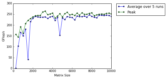
For context, here are some other results:
- A 16 core Intel Xeon E5-2630 v3 node running on Sheffield’s HPC system achieved around 500 Gigaflops.
- My mid-2014 Mabook Pro, with a Haswell Intel CPU hit, hit 169 Gigaflops.
- My Dell XPS9560 laptop, with a Kaby Lake Intel CPU, manages 153 Gigaflops.
As you can see, we are getting quite a lot of compute power for nothing from Azure Notebooks. Of course, one of the limiting factors of the free notebook service is that we are limited to 4GB of RAM but that was more than I had on my own laptops until 2011 and I got along just fine.
Another fun fact is that according to https://www.top500.org/statistics/perfdevel/, 263 Gigaflops would have made it the fastest computer in the world until 1994. It would have stayed in the top 500 supercomputers of the world until June 2003 [1].
Not bad for free!
[1] The top 500 list is compiled using a different benchmark called LINPACK so a direct comparison isn’t strictly valid…I’m using a little poetic license here.
There are lots of Widgets in ipywidgets. Here’s how to list them
from ipywidgets import *
widget.Widget.widget_types
At the time of writing, this gave me
{'Jupyter.Accordion': ipywidgets.widgets.widget_selectioncontainer.Accordion,
 'Jupyter.BoundedFloatText': ipywidgets.widgets.widget_float.BoundedFloatText,
 'Jupyter.BoundedIntText': ipywidgets.widgets.widget_int.BoundedIntText,
 'Jupyter.Box': ipywidgets.widgets.widget_box.Box,
 'Jupyter.Button': ipywidgets.widgets.widget_button.Button,
 'Jupyter.Checkbox': ipywidgets.widgets.widget_bool.Checkbox,
 'Jupyter.ColorPicker': ipywidgets.widgets.widget_color.ColorPicker,
 'Jupyter.Controller': ipywidgets.widgets.widget_controller.Controller,
 'Jupyter.ControllerAxis': ipywidgets.widgets.widget_controller.Axis,
 'Jupyter.ControllerButton': ipywidgets.widgets.widget_controller.Button,
 'Jupyter.Dropdown': ipywidgets.widgets.widget_selection.Dropdown,
 'Jupyter.FlexBox': ipywidgets.widgets.widget_box.FlexBox,
 'Jupyter.FloatProgress': ipywidgets.widgets.widget_float.FloatProgress,
 'Jupyter.FloatRangeSlider': ipywidgets.widgets.widget_float.FloatRangeSlider,
 'Jupyter.FloatSlider': ipywidgets.widgets.widget_float.FloatSlider,
 'Jupyter.FloatText': ipywidgets.widgets.widget_float.FloatText,
 'Jupyter.HTML': ipywidgets.widgets.widget_string.HTML,
 'Jupyter.Image': ipywidgets.widgets.widget_image.Image,
 'Jupyter.IntProgress': ipywidgets.widgets.widget_int.IntProgress,
 'Jupyter.IntRangeSlider': ipywidgets.widgets.widget_int.IntRangeSlider,
 'Jupyter.IntSlider': ipywidgets.widgets.widget_int.IntSlider,
 'Jupyter.IntText': ipywidgets.widgets.widget_int.IntText,
 'Jupyter.Label': ipywidgets.widgets.widget_string.Label,
 'Jupyter.PlaceProxy': ipywidgets.widgets.widget_box.PlaceProxy,
 'Jupyter.Play': ipywidgets.widgets.widget_int.Play,
 'Jupyter.Proxy': ipywidgets.widgets.widget_box.Proxy,
 'Jupyter.RadioButtons': ipywidgets.widgets.widget_selection.RadioButtons,
 'Jupyter.Select': ipywidgets.widgets.widget_selection.Select,
 'Jupyter.SelectMultiple': ipywidgets.widgets.widget_selection.SelectMultiple,
 'Jupyter.SelectionSlider': ipywidgets.widgets.widget_selection.SelectionSlider,
 'Jupyter.Tab': ipywidgets.widgets.widget_selectioncontainer.Tab,
 'Jupyter.Text': ipywidgets.widgets.widget_string.Text,
 'Jupyter.Textarea': ipywidgets.widgets.widget_string.Textarea,
 'Jupyter.ToggleButton': ipywidgets.widgets.widget_bool.ToggleButton,
 'Jupyter.ToggleButtons': ipywidgets.widgets.widget_selection.ToggleButtons,
 'Jupyter.Valid': ipywidgets.widgets.widget_bool.Valid,
 'jupyter.DirectionalLink': ipywidgets.widgets.widget_link.DirectionalLink,
 'jupyter.Link': ipywidgets.widgets.widget_link.Link}
This is my rant on import *. There are many like it, but this one is mine.
I tend to work with scientists so I’ll use something from mathematics as my example. What is the result of executing the following line of Python code?
result = sqrt(-1)
Of course, you have no idea if you don’t know which module sqrt came from. Let’s look at a few possibilities. Perhaps you’ll get an exception:
In [1]: import math
In [2]: math.sqrt(-1)
---------------------------------------------------------------------------
ValueError Traceback (most recent call last)
in ()
----> 1 math.sqrt(-1)

ValueError: math domain error
Or maybe you’ll just get a warning and a nan
In [3]: import numpy
In [4]: numpy.sqrt(-1)
/Users/walkingrandomly/anaconda/bin/ipython:1: RuntimeWarning: invalid value encountered in sqrt
#!/bin/bash /Users/walkingrandomly/anaconda/bin/python.app
Out[4]: nan
You might get an answer but the datatype of your answer could be all sorts of strange and wonderful stuff.
In [5]: import cmath
In [6]: cmath.sqrt(-1)
Out[6]: 1j
In [7]: type(cmath.sqrt(-1))
Out[7]: complex

In [8]: import scipy
In [9]: scipy.sqrt(-1)
Out[9]: 1j
In [10]: type(scipy.sqrt(-1))
Out[10]: numpy.complex128

In [11]: import sympy
In [12]: sympy.sqrt(-1)
Out[12]: I
In [13]: type(sympy.sqrt(-1))
Out[13]: sympy.core.numbers.ImaginaryUnit
Even the humble square root function behaves very differently when imported from different modules! There are probably other sqrt functions, with yet more behaviours that I’ve missed.
Sometimes, they seem to behave in very similar ways:-
In [16]: math.sqrt(2)
Out[16]: 1.4142135623730951

In [17]: numpy.sqrt(2)
Out[17]: 1.4142135623730951

In [18]: scipy.sqrt(2)
Out[18]: 1.4142135623730951
Let’s invent some trivial code.
from scipy import sqrt

x = float(input('enter a number\n'))
y = sqrt(x)

# important things happen after here. Complex numbers are fine!
I can input -1 just fine. Then, someone comes along and decides that they need a function from math in the ‘important bit’. They use import *
from scipy import sqrt
from math import *

x = float(input('enter a number\n'))
y = sqrt(x)

# important things happen after here. Complex numbers are fine!
They test using inputs like 2 and 4 and everything works (we don’t have automated tests — we suck!). Of course it breaks for -1 now though. This is easy to diagnose when you’ve got a few lines of code but it causes a lot of grief when there’s hundreds…or, horror of horrors, if the ‘from math import *’ was done somewhere in the middle of the source file!
I’m sometimes accused of being obsessive and maybe I’m labouring the point a little but I see this stuff, in various guises, all the time!
So, yeah, don’t use import *.
While waiting for the rain to stop before heading home, I started messing around with the heart equation described in an old WalkingRandomly post. Playing code golf with myself, I worked to get the code tweetable. In Python:
from pylab import *
x=r_[-2:2:0.001]
show(plot((sqrt(cos(x))*cos(200*x)+sqrt(abs(x))-0.7)*(4-x*x)**0.01)) pic.twitter.com/gbOTbYSaIG— Mike Croucher (@walkingrandomly) February 8, 2016
In R:
x=seq(-2,2,0.001)
y=Re((sqrt(cos(x))*cos(200*x)+sqrt(abs(x))-0.7)*(4-x*x)^0.01)
plot(x,y)#rstats pic.twitter.com/trpgEnNna4— Mike Croucher (@walkingrandomly) February 8, 2016
I liked the look of the default plot in R so animated it by turning 200 into a parameter that ranged from 1 to 200. The result was this animation:
Finding this animation based on previous tweets oddly mesmerising #rstats pic.twitter.com/e3q6lZqWcP
— Mike Croucher (@walkingrandomly) February 8, 2016
The code for the above isn’t quite tweetable:
options(warn=-1)
for(num in seq(1,200,1))
{
    filename = paste("rplot" ,sprintf("%03d", num),'.jpg',sep='')
    jpeg(filename)
    x=seq(-2,2,0.001)
    y=Re((sqrt(cos(x))*cos(num*x)+sqrt(abs(x))-0.7)*(4-x*x)^0.01)
    plot(x,y,axes=FALSE,ann=FALSE)
    dev.off()
}
This produces a lot of .jpg files which I turned into the animated gif with ImageMagick:
convert -delay 12 -layers OptimizeTransparency -colors 8 -loop 0 *.jpg animated.gif