
Archive for March, 2008
I work at the University of Manchester which is where the world’s first ever stored-program electronic digital computer was made back in 1948. It was originally called the Manchester Small Scale Experimental Machine but everyone called it Baby and it didn’t occur to it to mind. Before I get flamed to death by US computer historians – yes the ENIAC was built 2 years before Baby but it had a fundamentally different architecure (as explained by Alan Burlison in his blog – here). As Alan says, if you wanted to reprogram ENIAC, you needed a pair of pliars.
Many people who are a lot more eloquent than me have written a lot about the history of this machine (here for example) so I won’t say too much about it here except that it had only 128 bytes of memory which were arranged in 32 x 32 bit binary words and that it had an instruction set of only 7 commands which made programming it a bit tricky to say the least.
If you think you are a real programmer who is up to the challenge of coding for a 60 year old machine then Manchester University is holding a program “The Baby” competition (closing date 1 May 2008) to celebrate the Baby’s 60th anniversary. There is a photo realistic Java-based simulator of the machine, complete with example programs, over at the competition website along with an instruction manual to get you started. With only 7 instructions to learn how hard can it be?
Say you have just joined an applied-maths research group* where you are expected to write a lot of numerical simulations – numerical simulations that are going to require the use of big computers in large, air conditioned rooms with a great deal of impressive looking flashenlightenblinken. Naturally, you would like to use Python for all of your programming needs as you have recently fallen in love with it and you are convinced that it’s the future.
Your boss, Bob, completely disagrees with your take on the future of programming. He thinks that Python is a passing fad that will soon be forgotten. He sneeringly refers to it as a ‘ mere scripting language’ and constantly refers to you as the script kiddie. He thinks that Fortran is the only programming language worth bothering with when it comes to numerical simulations. According to Bob, Fortran is the past, present and future of computer programming – everything else is just mucking about.
You argue constantly with Bob concerning the relative merits of the two languages because, although you respect Fortran, you don’t think that it’s going to be much fun to use. Eventually he pulls out his trump card – “You can’t use Python in this group because all of our screamingly fast, highly accurate, tested and debugged numerical routines are written in Fortran. We won’t use any other libraries because these are the best so – give up on Python and start learning Fortran or get another job.”
Defeated…or so you thought…
After a bit of googling you realize that there is light at the end of the tunnel, this problem has been solved before by making use of the Python ctypes module. First of all let’s install this module on Ubuntu:
sudo apt-get install python-ctypes
Taking our cue from this solution lets say that one of the functions in the Fortran library is called ADD_II and has the following source code (filename add.f)
SUBROUTINE ADD_II(A,B)
INTEGER*4 A,B
A = A+B
END
Compile it into a shared library using gfortran as follows:
gfortran add.f -ffree-form -shared -o libadd.so
Now, create a file called add.py and copy the source code from our friendly usenet poster:
from ctypes import *
libadd = cdll.LoadLibrary(“./libadd.so”)
#
# ADD_II becomes ADD_II_
# in Python, C and C++
#
method = libadd.ADD_II_
x = c_int(47)
y = c_int(11)
print “x = %d, y = %d” % (x.value, y.value)
#
# The byref() is necessary since
# FORTRAN does references,
# and not values (like e.g. C)
#
method( byref(x), byref(y) )
print “x = %d, y = %d” % (x.value, y.value)
run the script as follows:
python add.py
and get the following error message:
AttributeError: ./libadd.so: undefined symbol: ADD_II_
So, despite what we may have thought, it looks like our function has not been given the name ADD_II_ in the shared library. So what name has it been given? We could just keep guessing what the compiler might have called it or we could just ask the library itself using the nm comand:
nm libadd.so
00001468 a _DYNAMIC
00001554 a _GLOBAL_OFFSET_TABLE_
w _Jv_RegisterClasses
00001458 d __CTOR_END__
00001454 d __CTOR_LIST__
00001460 d __DTOR_END__
0000145c d __DTOR_LIST__
00000450 r __FRAME_END__
00001464 d __JCR_END__
00001464 d __JCR_LIST__
00001570 A __bss_start
w __cxa_finalize@@GLIBC_2.1.3
00000400 t __do_global_ctors_aux
00000340 t __do_global_dtors_aux
00001568 d __dso_handle
w __gmon_start__
000003d7 t __i686.get_pc_thunk.bx
00001570 A _edata
00001574 A _end
00000434 T _fini
000002d8 T _init
000003dc T add_ii_
00001570 b completed.6030
000003a0 t frame_dummy
0000156c d p.6028
Now I have no idea what most of that output means but it looks like the .so file contains something called add_ii_ so if I use this instead of ADD_II_ in my python script I bet it will work.
python add.py
x = 47, y = 11
x = 58, y = 11
The sweet smell of success. You go to Bob and tell him that you have just come up with a test script that demonstrates that you are going to be able to use the group’s Fortran libraries in your Python scripts.
“That’s very nice” says Bob “but all of the really useful routines in the library make use of callback functions. Can you handle those yet?”
“yes I can” you reply smugly “but this post has gone on long enough so I’ll leave the details until another time”
*Note – In case you are my boss – I haven’t joined a research group so I won’t be quitting my job any day soon. I was just in a story telling mood. Oh..and this stuff will be useful for what we do – I promise!
If you work in the field of Chemistry then it’s highly likely that you will want to produce Lewis Dot diagrams at some point in your career. If you have never heard of them then essentially what they do is show the distribution of electrons in atoms and molecules in schematic form. For example, the diagram below is the Lewis dot diagram for ethane (original source here)
Over at the Teaching College Math Technology Blog, Maria has produced a tutorial video that shows how to produce these diagrams using Design Science’s MathType. In addition she has posted a second tutorial that has been produced by an employee of Design Science – well worth a look if this is something you need to do.
The 29th edition of the Carnival of Mathematics has been posted over at quomodocumque. Topics include group theory, game theory, the Collatz conjecture and much more.
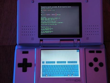
Not too long ago it was necessary to buy some rather expensive hardware if you wanted access to a computer algebra system. The first time I used Mathematica (back in 2000), for example, it was installed on a Unix machine, shared between about 30 researchers, which cost around 8000 pounds! These days of course, it runs quite happily on a laptop costing just a few hundred pounds but now it’s even possible to get access to a computer algebra system on a hardware as cheap as a handheld games console!
The computer algebra system in question is Mathomatic, an open source application that has been in continuous development for over 20 years. It’s capable of acting as a calculator, solving and simplifying equations and doing calculus on polynomials among other things. Back in late 2006 it was ported over to Nintendo’s DS console – twice!. I haven’t had chance to try it out because I don’t own the hardware (story of my life) but I would love to hear from anyone who has played with it (or any other maths package for that matter) on one of these game consoles.
Nintendo’s machine is already being used in an educational setting (successfully it seems although much larger trials need to be done I think) using Dr Kawashima’s More Brain Training which apparently helps with skills such as mental arithmetic, memory and problem solving but I think this is just scratching the surface of what can be done with this kind of technology.
What would be really amazing would be a port of Wolfram’s Mathplayer to a device like this – then the Wolfram Demonstrations project would definitely come into its own. I imagine that the Nintendo DS (or the iPhone for that matter) doesn’t have enough computational power to successfully run something as complicated as Mathplayer but I think that affordable handheld devices that do are just around the corner.
In a recent post I asked if anyone had any requests for any Wolfram Demonstrations that they would like to see made. Maria Andersen of the Teaching College Math Technology Blog requested a demonstration that would produce music from the decimal expansion of rational numbers in the same way that this one does for irrational numbers. Well, I always aim to please so here it is:
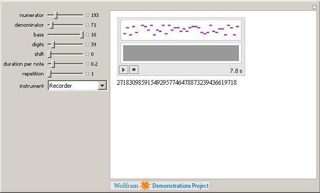
Just set the numerator and denominator with the sliders, choose the base of the result, the number of digits etc, along with what instrument you want and then click play. Remember, if you don’t have Mathematica then you can always use their free MathPlayer to run this demonstration. I hope this is what you were looking for Maria but if it isn’t then let me know what you would like changed and I will see what I can do.
If anyone else has any Wolfram Demonstration requests then leave a comment and I might just code it up for you (unless someone beats me to it of course).
1.Take one dare from Kathryn Cramer and obtain a picture from her website.
2. Steal ideas from this demonstration by Jeff Bryant.
3. Type the following incantations into Mathematica
SetDirectory[“/home/mike/Desktop/random”];
image = Import[“kramer.jpg”];
xpos[x_] := Floor[x/N[2/374.] + 377/2.]
ypos[x_] := Floor[x/N[2/499.] + 502/2.]
imcol[x_, y_] := image[[1]][[1]][[xpos[x]]][[ypos[y]]]/256.;
a = 1; b = 0.9; c = 1;
Plot3D[{Sqrt[ c^2*(1 – (x^2/a^2 + y^2/b^2))], -Sqrt[c^2*(1 – (x^2/a^2 + y^2/b^2))]}, {x, -1, 1}, {y, -1, 1}, ColorFunction -> (RGBColor[imcol[#1, #2]] &), Boxed -> False, Axes -> False, AspectRatio -> 2, ViewAngle -> Pi/13, ViewPoint -> {-3.00336, 0.86708, 3.14159}, PlotRange -> All, Mesh -> False, PlotPoints -> 400]
Enjoy!

I have been playing with the new release of Mathematica for a little while now and thought that I would share what I have found. Now, as indicated by the small increment in version number, this is a minor release and so we should not be expecting anything earth shattering. The sort of things that one expects in a minor release like this include things such as bug-fixes, small performance enhancements, documentation upgrades etc. So…let’s see what he have got.
First on the list are some changes to the documentation center. Copying and pasting from Wolfram’s press release:
- New Virtual Book documentation with updated Mathematica Book content
- New Function Navigator, an easily browsable overview of all Mathematica objects
Let’s start with the Virtual book – what’s that all about? Like Gavin Scott, the writer of this forum message, I went to the help browser and searched for ‘virtual book’ hoping to be enlightened. Nothing – not a single search result! I found this surprising since Wolfram Research felt that it was such an important modification that they chose it to be the first thing they mentioned on their press release. To be honest I probably would not have noticed the new virtual book icon in the help browser without Gavin’s help. To help you find it I have circled it in red in the image below

Clicking on this icon opens the virtual book itself (see the image below) which is essentially an alternative way to navigate the documentation system. This might not seem like much to the casual observer but since the release of version 6 many people have been complaining about the changes made in the documentation system since version 5.2. The Virtual Book is Wolfram’s attempt at addressing some of these complaints by adding some structure that is reminiscent of the original Mathematica Book and I don’t think its too bad at all.
Personally, I have gotten used to the new Documentation center and, although I feel it has some problems, I quite like it – especially the huge number of examples that it contains. However, it does contain a massive quantity of information which is sometimes difficult to navigate through so the extra layer of structure that the Virtual Book provides is a welcome addition.
Next up we have the Function Navigator (below) which, like the Virtual Book, is yet another way to navigate through the documentation. Now this is something that I feel will be very useful – particularly when you are exploring a new area of functionality in Mathematica.
Say that you need to do some statistical calculations and you want to see what functions are available to you in Mathematica. Start off by expanding Mathematics and Algorithms followed by statistics to reveal the window below.

Clicking on our area of interest (Random Number Generation say) will reveal all of the functions available in that area. This is a very useful addition to the help system in my opinion. One minor issue with both the Virtual Book and the Function Navigator is that the windows take longer than expected to initialize. I conducted all of my tests on a pretty fast dual core machine with 4gb RAM and it took almost 3 seconds for the window to appear from the instant I clicked on the icon. I imagine that it is going to be painfully slow on my laptop which has a much lower specification but I haven’t tested it yet. At least one other person has noticed this issue.
The next item on Wolfram’s press release is
- Several additional documentation enhancements, including performance improvements, indexing, and link trails
I simply cannot comment on this as they have not given any examples and I cannot see any obvious changes. Would anyone care to enlighten me? Moving on…
- Full 64-bit performance on Intel Macs
This is great news if you are an owner of an Intel Mac but I’m not so onto the next item.
That’s great but it would be even better if Wolfram were more specific on this. There are some extra details on Wolframs blog post concerning 6.0.2 but even that doesn’t tell the full story. Quoting from Wolfram’s blog:
“A few examples are dramatic compression of graphics that include transparency exported to PDF, more robust embedding of graphics in TeX, and full support for all metadata in FITS images.”
What I would have really liked to have seen here is a comprehensive list of the improvements made – not just a select few. The next few points on Wolfram’s list are all related to the above
- Significant speedup in import of binary data files
- Improved handling of graphics when exporting to TeX and PDF
- Enhanced import of metadata from FITS astronomical image files
The final point Wolfram makes about this new release is
- New coordinate-picking tool and improved highlighting of graphical selections for interactive graphics
This is discussed in detail in the Wolfram’s blog so I will leave it to them to explain what this new feature is. In short – it’s fantastic! I may blog about it myself soon as it looks like it might be extremely useful.
That pretty much covers everything that Wolfram has released concerning this update and apart from the changes in the documentation (which are welcome improvements) it all seems a bit vague to me. I am the administrator for a large university site license and already I have people asking me if the upgrade is worth it if you are coming from version 6.0.1. My current response is along the lines of “well for us its essentially free (more accurately we have paid for it in advance) so you may as well” but if I had to pay extra for it then I probably wouldn’t bother.
The reason that I wouldn’t bother to pay for an upgrade is not because I think it is a bad product – quite the opposite in fact as it is a superb product – but if one is happily using version 6.0 or 6.0.1 then Wolfram Research simply haven’t given us the information we need to decide if we should upgrade or not.
With a bit of googling I eventually came up with some more details that I wished Wolfram would have released publicly. All of the following have been gleaned from posts to newsgroups.
csv files – original source -> here
There is a subtle change in the way .csv files are imported at 6.02.
Put the following into a .csv file:
“hope”
1
2
At 6.01 (and earlier versions of Mathematica) the string was read in as
“hope”. At 6.02 the quotes are included in the string – “\”hope\””.
Integration bug fix – original source -> here
N[Integrate[Log[z] Log[1 + Sqrt[1 – z^2]], {z, 0, 1}]] = -0.707202 (version 6 – incorrect)
N[Integrate[Log[z] Log[1 + Sqrt[1 – z^2]], {z, 0, 1}]] = -0.659589 (version 6.0.2 – correct)
Various improvements – original source -> here
- Fix for a big slowdown in FactorInteger
- Fixes for some wrong Integrate results pointed out by external users
- A few Series fixes
- A few Simplify/FullSimplify/FunctionExpand fixes
- Faster and more reliable numericizing of MeijerG
- A few fixes in special function evaluation
- Fix for RamanujanTau with large arguments
That’s the sort of thing I want to see – details.
I want to see a big list of bug fixes so that I can point to them and say to a user “the new version fixes all of these – if they affect you then you need to upgrade”
I want to see a list of performance enhancements so that I can point to them and say to a user “the new version is faster in all of these areas – if you need them then you need to upgrade”
I want to see a list of changes in function behaviour (such as the csv example above) so that I can explain to someone why their 6.0.1 code no longer works in 6.0.2 without spending all night figuring out some undocumented change.
I don’t have any of this information so all I can do is say “You may as well upgrade I guess – the documentation navigation has been improved a bit. It probably won’t do any harm (unless they have changed the way a function works without documenting it – see the csv example above)” Its hardly compelling is it?
Please Wolfram, give me more details. I like details and so do a lot of other people who are wondering whether or not to part with their hard-earned cash for this release.
Mathematica 6.0.2 was released back on February 25th but I have only just managed to find the time to install it. I tried to install it on a brand new Dell 755 with a very fresh install of Ubuntu but near the end of the install procedure I came across the following error
“The installer was unable to check for a valid password file. Your Mathematica installation may be incomplete or corrupted.”
I had not been given the opportunity to supply it with any licensing information so it looked like there was a problem with the installer itself. Cutting a long story sort, the solution is to use apt to install the package libstdc++5 as follows
sudo apt-get install libstdc++5
This is a very common package and I guess that I have not seen this error before because libstdc++5 is automatically installed as a prerequisite for many other Ubuntu applications. Hopefully this little note will be of use to a googler or two.
Anyway…I now have 6.0.2 installed and running so expect a breakdown of the new features soon.
Next Friday will be March 14th which is celebrated by some as Pi Day since the date is 3/14 in American date format and the first three digits of Pi are 3.14 (as if I have to tell you!). One or two people have been looking for inspiration as to what to do for Pi Day in schools and I thought that it would be fun to write a Wolfram Demonstration especially for Pi Day, after all, my Valentine’s day demonstrations turned out to be quite popular.
So the question that remained to be answered was “what demonstration should I write?”
I have already written a post about making music out of the digits of Pi and discovered that a great demonstration had been written by Hector Zenil so there was no point in thinking about that.
How about Buffon’s needle? That’s a fun problem that leads to an approximation of Pi. Unfortunately for me – this is a demonstration that has already been written.
Perhaps I could do something that looked at the randomness in the digits of Pi? After all – this blog IS called walking randomly and I haven’t looked at randomness very much yet. Unfortunately I have been beaten to this one too (By Stephen Wolfram himself no less).

My next thought was to consider some series that would sum up to approximations of Pi. Again – it’s been done.

In addition to these three there are many others such as
- Consecutive Digits in the Expansion of Pi
- Pi Digits Bar Chart
- Pi Digits Pie
- Wallis’ Sieve Pi Approximation
- Graphs Of Successive Digits Of Pi, E and Phi
- Wallis Formula
That’s a lot of Pi and I have only just gotten started. All in all I am stumped – I have no idea of a demonstration I might write for Pi Day but if you can think of something then let me know and I will see what I can do :) (Oh and I will make sure that you get credit for your idea when I submit it to the project)