
Archive for January, 2011
I tend to keep an eye out for news relating to mathematical software and thought that I’d start sharing my monthly notebook with the world in case it proved to be useful to anyone else. If you have any math-software news that you’d like to share then feel free to contact me.
Releases – Commercial
Mathcad Prime 1.0 has been released by PTC who have almost completely rewrote it from scratch. Interestingly, you get a version of Mathcad 15.0 thrown in for free when you buy a copy. See my discussion of this new version here.
MAGMA v2.17-3 has been released and the changelog is here. Magma is a large software package designed for computations in algebra, number theory, algebraic geometry and algebraic combinatorics.
Version 12 of the popular plotting package, Sigmaplot, has been released. The press release is at www.sigmaplot.com/aboutus/pressroom_details.php?link=jan-2010
Releases – Open Source
A bug-fix version of Matplotlib has been released – version 1.0.1 – and the changelog is available on sourceforge. Matplotlib is a 2D plotting library for Python.
SAGE 4.6.1 has been released. The detailed changelog is here. SAGE’s mission is “Creating a viable free open source alternative to Magma, Maple, Mathematica and Matlab.”
deal.II version 7 has been released. deal.II is a C++ program library targeted at the computational solution of partial differential equations using adaptive finite elements.
JQuantlibLib version 0.2.4 released. Details here. JQuantLib is a BSD Licensed, open-source, comprehensive framework for quantitative finance, written in Java.
Mobile Math Software
Wolfram Research have released a trio of iPhone apps called Course Assistants. Essentially these are nice user interfaces to Wolfram Alpha that make it easier to use in specific subject domains. The initial offering consists of Algebra, Calculus and Music Theory. Stephen Wolfram has blogged about the new apps.
MATLAB software community
The Mathworks have launched a MATLAB-specific question and answer site called MATLAB Answers. In conjunction with the venerable comp.soft-sys.matlab newsgroup and the more recent Stack Overflow, MATLABers now have more question and answer resources than ever. The Matworks have a blog article about the new service.
New Books
Introduction to Scientific Computing by Victor Eijkhout. You can download it for free or get a printed copy for under 12 pounds.
So here’s a fun (and potentially useful) probability puzzle for you all to ponder. Here in the UK we have an investment option called Premium Bonds. From the premium bonds website:
“Premium Bonds are an investment where, instead of interest payments, investors have the chance to win tax-free prizes. When someone invests in Premium Bonds they are allocated a series of numbers, one for each £1 invested.”
There’s a prize draw every month and a range of prizes from 25 pounds right up to 1 million pounds. You can get your money back at any time with no penalty. So, if you invest 1000 pounds then you get 1000 shots at winning a prize every month for as long as you leave the investment alone. More detailed information such as odds etc is available here.
The way I like to think of premium bonds is that they are a bit like the National Lottery (click here for discussion of odds) except that you get your money back after you’ve played. So I was thinking that, instead of buying premium bonds, an alternative investment strategy would be to put all of your money into a high interest cash account (paying N% per year) and use the resulting interest to buy lottery tickets.
Both strategies offer similar security (you can get your principle investment back at any time) and both of them are a bit of fun since they are based on games of chance. Assuming I am to choose one of these strategies, which one is going to offer me the best rate of return over the long term?
MATLAB’s control system toolbox has functions for converting transfer functions to either state space representations or zero-pole-gain models as follows
%Create a simple transfer function in MATLAB
num=[2 3];
den = [1 4 0 5];
mytf=tf(num,den);

%convert this to State Space form
tf2ss(num,den)
ans =

0   1   0
0   0   1
-5  -0  -4

%Convert to zero-pole-gain form
[z,p,k]=tf2zp(num,den)
z = -1.5000
p =

-4.27375 + 0.00000i
0.13687 + 1.07294i
0.13687 - 1.07294i

k =  2
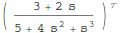
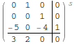
Now that Mathematica 8 is available I wondered what the Mathematica equivalent to the above would look like. The conversion to a StateSpace model is easy:
mytf=TransferFunctionModel[(2 s + 3)/(s^3 + 4 s^2 + 5), s]
StateSpaceModel[mytf]
but I couldn’t find an equivalent to MATLAB’s tf2zp function.
I can get the poles and zeros easily enough (as an aside it’s nice that Mathematica can do this exactly)
TransferFunctionPoles[mytf]
TransferFunctionZeros[mytf]
but what about gain? There is no TransferFunctionGain[] function as you might expect. There is a TransferFunctionFactor[] function but that doesn’t do what I want either.
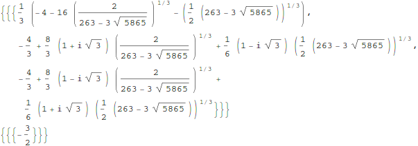
It turns out that there is a function that will do what I want but it is hidden from the user a little in an internal function
Control`ZeroPoleGainModel[mytf]

Control`ZeroPoleGainModel[{{{{-(3/2)}}}, {1/
     3 (-4 - 16 (2/(263 - 3 Sqrt[5865]))^(
        1/3) - (1/2 (263 - 3 Sqrt[5865]))^(1/3)), -(4/3) +
     8/3 (1 + I Sqrt[3]) (2/(263 - 3 Sqrt[5865]))^(1/3) +
     1/6 (1 - I Sqrt[3]) (1/2 (263 - 3 Sqrt[5865]))^(1/3), -(4/3) +
     8/3 (1 - I Sqrt[3]) (2/(263 - 3 Sqrt[5865]))^(1/3) +
     1/6 (1 + I Sqrt[3]) (1/2 (263 - 3 Sqrt[5865]))^(1/3)}, {{2}}}, s]
That’s not as user friendly as it could be though. How about this?
tf2zpk[x_] := Module[{z, p, k,zpkmodel},
  zpkmodel = Control`ZeroPoleGainModel[x];
  z = zpkmodel[[1, 1, 1, 1]];
  p = zpkmodel[[1, 2]];
  k = zpkmodel[[1, 3, 1]];
  {z, p, k}
  ]
Now we can get very similar behavior to MATLAB:
In[10]:= tf2zpk[mytf] // N

Out[10]= {{-1.5}, {-4.27375, 0.136874 + 1.07294 I,
  0.136874 - 1.07294 I}, {2.}}
Hope this helps someone out there. Thanks to my contact at Wolfram who told me about the Control`ZeroPoleGainModel function.
Other posts you may be interested in
A man I have a lot of time for is Joel Spolsky, author, software developer and previously a program manager for Microsoft Excel. Way back in the year 2000 he wrote an article called Things You Should Never Do, Part 1 where his main point was “The single worst strategic mistake that any software company can make is to rewrite your code from scratch.” He exemplified this principle using products such as Quattro Pro and Netscape 6.0.
Not everyone agrees with Joel’s thesis and it seems that the managers at PTC, the owners of Mathcad, are among them. The last major update of Mathcad was version 14.0 which was released back in 2007 (the recent Mathcad 15.0 was a relatively minor update despite the .0 version number). To some outsiders it appeared that PTC were doing very little with the product until it transpired that what they were actually doing was an almost complete rewrite from the ground up.
That rewrite has now been released in the form of Mathcad Prime 1.0. I don’t have my hands on a copy yet so I have been scouring the web to try and determine exactly what this new version does right and what it does wrong. Here’s what I’ve found so far.
- Mathcad Prime 1.0 does not have everything that Mathcad 15 has. Jackov Kucan, Director of development at PTC, has publicly stated that it won’t be until Prime 3.0 that users will be able to retire Mathcad 15 and migrate to Prime.
- Relating to the above point,there is a thread over at the PTC Forums where several users are calling Mathcad Prime a big step backwards. Not everyone agrees though.
- Another useful discussion thread is one started by PTC where they ask What new features do you want to see in Mathcad Prime?
- According to one of the discussion threads above, Mathcad Prime doesn’t include several pieces of functionality (symbolics, 3d graphs and animation) that are considered bog standard by competitors such as Maple and Mathematica. I haven’t confirmed this yet. (confirmed by email from a PTC employee)
- At the time of writing, all purchasers of Mathcad Prime 1.0 will also receive Mathcad 15. Mathcad Prime 1.0 can be installed side by side with any previous versions of Mathcad. (source)
- In the UK, Mathcad Prime currently costs £810 for a personal license. (source)
Here’s a nice demo of the new version by Jackov Kucan. The user interface looks great in my opinion although I confess to not being a fan of the Microsoft-like ribbon interface.
How about you? Have you used MathCAD prime yet? If so then what do you think of it? If not then do you think you will try it?
Update (16th February 2011): I was recently contacted by an employee of PTC who told me ‘The internal engine has not been totally rewritten . It’s the user interface, which includes the equation editor and plots that we rebuilt from scratch.’ Thanks for the clarification.
If you like this post then you may also be interested in the following:
- Free Mathcad alternative, Smath studio, updated. Now with units!
- Mathcad Prime Screenshots – From an early beta version
MATLAB 2010b was released a couple of months ago and, as usual, it comes with a whole range of new features, performance enhancements and all important bug fixes. Within the MATLAB 2010b documentation, there are lists of the new functionality but I like to dig in a bit deeper and pick out one or two things that are of personal interest to me.
64 bit integer support
Back in April 2010, I was working with the NAG Toolbox for MATLAB which makes use of 64 bit integers on 64 bit machines and I learned that MATLAB 2010a and earlier didn’t support even the most basic of operations on 64 bit integers. For example, on MATLAB 2010a:
a=int64(10);
b=int64(20);
a+b
??? Undefined function or method 'plus' for input arguments of type 'int64'.
I’m happy to report that this has now been fixed and The Mathworks have implemented 18 basic operators for 64bit integer types including arithmetic, the colon operator, bsxfun and more. This has made my life (and the lives of some of the people I support) MUCH easier and I really appreciate The Mathworks work on this one.
Curve Fitting and Splines toolboxes merged
MATLAB has got a lot of toolboxes. In fact, it’s got far too many in my opinion which makes the product more expensive and fragmented. I have literally lost count of the amount of times someone has emailed me with a query like “I don’t suppose you have access to the XYZ toolbox because someone had sent me code that uses it and I can’t run it’ Quite frankly, it sucks.
So, when The Mathworks announce that they are merging the functionality of two related toolboxes into one, there is much rejoicing in Walking Randomly towers. If The Mathworks would like to do some more toolbox merging then I have a couple of suggestions :)
CUDA support in the Parallel Computing Toolbox
These days, the hotness in research computing is to do as much of your calculation as possible on your graphics card. If handled correctly, the hunk of silicon that was originally designed to make games look pretty can speed up scientific calculations hundreds of times compared to dull old CPUs. There is a great deal of interest in GP-GPU programming at Manchester University (my employer), so much so that we have set up a GPU-Club for our researchers.
Arguably, the leader in GP-GPU (General Purpose – Graphics Processing Unit) hardware is NVIDIA who are the developers of the CUDA programming framework. Until now, CUDA support in MATLAB has been provided by third-parties such as Jacket (Commerical) or GP-You (free) but as of 2010b, there is now official support for CUDA GPUs in MATLAB’s parallel computing toolbox. At the moment, it is not as well developed as products such as Jacket but I would lay bets that this will change in the not too distant future.
My early experiments with this new functionality have met with zero success but I have new hardware on the way and I am really looking forward to getting my teeth into this.
Parallel Statistics
Parallel computing in MATLAB is more complicated than it should be. Some functions make use of multicore processors automatically and you don’t need the parallel computing toolbox to feel the benefit. On the other hand, there are an increasing number of functions in toolboxes such as statistics and optimisation, that additionally require the PCT in order to make maximum use of modern hardware.
The 2010b version of the statistics toolbox includes an extra 8 functions (candexch, cordexch, daugment, dcovary, nnmf, plsregress, rowexch and sequentialfs) that now make use of the PCT. If you have the PCT, then this is wonderful news but if you don’t then there is nothing to see here.
Faster trig functions when the argument is in degrees
The standard trigonometric functions such as sin, cos, tan and the like all work in radians but MATLAB also has several functions that accept their arguments in degrees: sind, cosd and tand for example. In MATLAB 2010b these functions have been made significantly faster. Lets see how much faster using my 3Ghz quad Core 2 Q9650 running Ubuntu 9.10
In MATLAB 2010a
x=rand(1,1000000)*360;
>> tic;y=cosd(x);toc
Elapsed time is 0.120207 seconds.
In MATLAB 2010b
x=rand(1,1000000)*360;
>> tic;y=cosd(x);toc
Elapsed time is 0.021256 seconds.
A speed up of around 5.6 times! What’s more, I’ve already come across a user’s code in the wild where this optimisation made a real difference to their execution time. As far as I can tell, the speed up comes from the fact that 2010a and below uses MATLAB code for these functions whereas 2010b and above uses mex files.
What other bloggers say about MATLAB 2010b
73 is an awesome number. In fact, one could argue that it’s the Chuck Norris of numbers. Here’s why (courtesy of Wikipedia, and Number Gossip):
- The mirror of 73, the 21st prime number, 37, is the 12th prime number. The number 21 has factors 7 and 3.
- In binary, 73 is a palindrome – 1001001
- Of the 7 binary digits representing 73, there are 3 ones.
- Every positive integer is the sum of at most 73 sixth powers.
- In octal, 73 is a repdigit – 111
- Pi Day occurs on the 73rd day of the year (March 14) on non-leap years
- 73 is the largest integer with the property that all permutations of all its substrings are primes
- 73 is the largest two-digit Unholey prime: such primes do not have holes in their digits
- 73 is the smallest number (besides 1) which is one less than twice its reverse
- 73 is the alphanumeric value of the word NUMBER: 14 + 21 + 13 + 2 + 5 + 18 = 73
73 is also the edition number of this, the latest Carnival of Mathematics, to which I bid you welcome. On with the show.
First up we have a mathematical calendar for 2011 courtesy of Ron Doerfler which focuses on Lightning Calculations. I have written about Ron’s calendar before and highly recommend it to all.
The beginning of a new calendar year is an opportunity for all of us to sit back and take stock of everything that took place over the previous 12 months. As a result you’ll find retrospectives of all kinds scattered around the internet and on TV such as The Best Tech Products of 2010, TV’s 11 best Watercooler Moments of the Year and so on. Over at his blog, Wild About Math, Sol Lederman points us to a much more mathematical restrospective of the year 2010 by giving us a heads up about an awesome looking new book.
Next we have the 2011 Mathematics game from Denise of Let’s Play Math; the rules of which can be most simply stated as “Use the digits in the year 2011 to write mathematical expressions for the counting numbers 1 through 100.” Head over there to see more detailed rules, hints, tips, discussion and solutions found so far.
If all of that isn’t quite enough to sate your appetite for all things 2011 then I suggest that you take a look at Patrick Vennebush’s post entitled 2011 – Prime Time which inspired Brent Yorgey to follow up with Prime Time in Haskell. I wonder if 2012 will inspire such mathematical and computational outpourings?
In her post, Two Planes, Tanya Khovanova stumbled across a seemingly innocent looking question in an old edition of Mathematics Teacher which made her take a deep breath and exclaim ‘Ooh, boy!’. Check it out to see what all the fuss is about.
In Redefining Great Britain, GrrlScientist highlights some new research that describes a clever way to redefine and redraw geographical areas using telephone communication networks — it relies on statistics and computing power.
Sander Huisman has a crack at inventing his own fractal based upon the q-gamma function using Mathematica and a heap of computer time. The resulting fractal zoom looks great. He’s also produced a really neat animation of a hinged tesselation.

How do you abbreviate the word ‘Mathematics’? Some say ‘math’ others say ‘maths’ but which came first and which is the most popular? In his post, Math/Maths in Google Books Ngrams, Peter Rowlett uses Google Ngrams to sample millions of books in order to try and determine the answer to these and similar questions.
The trapezoidal rule for numerical integration has been in the news recently and so John Cook of The Endeavour shows us Three surprises with the trapezoid rule.
Imagine that we want to bet on an event with m >= 2 possible outcomes, and that there are n >= 2 bookmakers taking bets on those outcomes. Note that the odds are known at the time the bets are placed, i.e., we have fixed-odds betting instead of pari-mutuel betting. We would like to know how to allocate our (limited) money, i.e., how much to bet on each outcome at each bookmaker. As we cannot foresee the future, we would very much like to lock in risk-less profits. In other words, we would like to find arbitrage opportunities (aka: “arbs”). In his post, Fixed-Odds Betting Arbitrage, Rod Carvalho discusses how, given the (fixed) odds posted by n bookmakers, we can detect the existence of arbitrage opportunities.
PhD student, Gianluigi Filippelli, considers a problem from way back in the 13th century in his post Fibonacci, Bombelli and imaginary numbers. Personally, I’ve always loved some of the historical aspects of mathematics and hope to attend a good course on it some day.
Finally, we have a post from Guillermo Bautista called Chess and the Axiomatic Systems where he provides an intuitive introduction to the notion of axiomatic systems through chess rules.
That’s it for this time but if you still need more mathematical blogging then check out The 12 Math Carnivals of 2010 and don’t forget to submit your articles to the forthcoming Math Teachers at Play carnival.
Follow the Carnival of Math on Twitter: @Carnivalofmath
Someone recently contacted me with a problem – she wanted to use MATLAB to perform a weighted quadratic curve fit to a set of data. Now, if she had the curve fitting toolbox this would be nice and easy:
x=[ 1 2 3 4 5];
y=[1.4 2.2 3.5 4.9 2.3];
w=[1 1 1 1 0.1];

f=fittype('poly2');
options=fitoptions('poly2');
options.Weights=[1 1 1 1 0.1];
fun=fit(x',y',f,options);
p1=fun.p1;
p2=fun.p2;
p3=fun.p3;

myfit = [p1 p2 p3]

myfit =
   -0.1599    1.8554   -0.5014
So, our weighted quadratic curve fit is y = -0.4786*x^2 + 3.3214*x – 1.84
So far so good but she didn’t have access to the curve fitting toolbox so what to do? One function that almost meets her needs is the standard MATLAB function polyfit which can do everything apart from the weighted part.
polyfit(x,y,2)
ans =
   -0.4786    3.3214   -1.8400
which would agree with the curve fitting toolbox if we set the weights to all ones. Sadly, however, we cannot supply the weights to the polyfit function as it currently stands (as of 2010b). My solution was to create a new function, wpolyfit, that does accept a vector of weights:
wpolyfit(x,y,2,w)
ans =
   -0.1599    1.8554   -0.5014
So where is this new function I hear you ask? Normally this is where I would provide you with a download link but unfortunately I created wpolyfit by making a very small modification to the original built-in polyfit function and so I might be on dicey ground by distributing it. So, instead I will give you instructions on how to make it yourself. I did this using MATLAB 2010b but it should work with other versions assuming that the polyfit function hasn’t changed much.
First, open up the polyfit function in the MATLAB editor
edit polyfit
change the first line so that it reads
function [p,S,mu] = wpolyfit(x,y,n,w)
Now, just before the line that reads
% Solve least squares problem.
add the following
w=sqrt(w(:));
y=y.*w;
for j=1:n+1
    V(:,j) = w.*V(:,j);
end
Save the file as wpolyfit.m and you are done. I won’t go over the theory of how this works because it is covered very nicely here. Comments welcomed.
2010 was a great year for mathematical blogging and this was reflected in the monthly Carnivals of Mathematics. Here they are again in case you missed them.
- January – 61st Carnival at Walkingrandomly
- February – 62nd Carnvial at The Endeavour
- March – 63rd Carnival at Mathrecreation
- April – 64th Carnival at Teaching College Math
- May – 65th Carnival at Maxwell’s Demon
- June – 66th Carnival at Wild About Math
- July – 67th Carnival at Travels in a Mathematical World
- August – 68th Carnival at Plus Magazine
- September – 69th Carnival at JD2718
- October – 70th Carnival at General Musings
- November – 71st Carnival at Theorem of the Day
- December – 72nd Carnival at 360
The cycle will be starting again next week when the 73rd carnival gets published right here at Walking Randomly. What happens after that is up to you because I need volunteers to host future editions. If you are interested then get in touch via the comments section of this post, via twitter or by email.
Links
- What is a maths carnival?
- Math Carnival submission form
- Math Teachers at Play – The sister carnival to CoM