Walking Randomly

This little corner of the web that I like to call home has been online for 4 years as of today.  I’d like to thank everyone who reads and comments on the stuff I put up here, I hope you find my wanderings interesting and/or useful.

I’d also like to thank all of the people and organisations I have collaborated with over the years while writing articles here. I’m not going to mention names out of fear of missing someone out but you know who you are.  The only exception would be Matthew Haworth of Reason Digital who talked me into starting this up during his University of Manchester farewell party.  He also provides me with web hosting (surviving three slashdottings so far), technical support and, on occasion, lunch!  Without Matt, there would be no Walking Randomly.

Back on WRs first birthday I gave out some stats (143 RSS subscribers and 250 visits per day) and so I’ll so the same today (1645 RSS subscribers and 800 unique visits per day)

Finally, here is a list of some of my favourite articles from over the last 4 years.  I hope you enjoy reading them as much as I enjoyed writing them

• Secret Messages hidden inside equations – When an equation literally spoke to me.
• The Valentine’s equations – Hearts and flowers, wrapped up in equations
• Now thats what I CALL Retro Computing – Ever wondered how easy it would be to program a 60 year old computer?  Now’s your chance
• Simulating Harmonographs – Pretty pictures from pendulums
• Proof I have a brain – When I blagged my way to a free brain scan
• Should Fortran be taught to undergraduates? – My first Slashdotting.  This post has been read by tens of thousands of people.
• Wheels on Wheels on Wheels – More pretty patterns
• The unreasonable ineffectiveness of factoring – We drill and kill the technique of factoring equations in schools.  A pity that its useless then!
• Polygonal numbers on quadratic number spirals – Yet more pretty patterns
• Math on iPad #1 – The beginning of a series that is still ongoing
• Quadraflakes, Pentaflakes, Hexaflakes and more – Playing with a particular kind of Fractal
• Complex Power Towers – recreations in the complex plane

This is part 2 of an ongoing series of articles about MATLAB programming for GPUs using the Parallel Computing Toolbox.  The introduction and index to the series is at https://www.walkingrandomly.com/?p=3730.   All timings are performed on my laptop (hardware detailed at the end of this article) unless otherwise indicated.

Last time

In the previous article we saw that it is very easy to run MATLAB code on suitable GPUs using the parallel computing toolbox.  We also saw that the GPU has its own area of memory that is completely separate from main memory.  So, if you have a program that runs in main memory on the CPU and you want to accelerate part of it using the GPU then you’ll need to explicitly transfer data to the GPU and this takes time.  If your GPU calculation is particularly simple then the transfer times can completely swamp your performance gains and you may as well not bother.

So, the moral of the story is either ‘Keep data transfers between GPU and host down to a minimum‘ or ‘If you are going to transfer a load of data to or from the GPU then make sure you’ve got a ton of work for the GPU to do.‘  Today, I’m going to consider the latter case.

A more complicated elementwise function – CPU version
Last time we looked at a very simple elementwise calculation– taking the sine of a large array of numbers.  This time we are going to increase the complexity ever so slightly.  Consider trig_series.m which is defined as follows

function out = myseries(t)
  out = 2*sin(t)-sin(2*t)+2/3*sin(3*t)-1/2*sin(4*t)+2/5*sin(5*t)-1/3*sin(6*t)+2/7*sin(7*t);
end

Let’s generate 75 million random numbers and see how long it takes to apply this function to all of them.

cpu_x = rand(1,75*1e6)*10*pi;
tic;myseries(cpu_x);toc

I did the above calculation 20 times using a for loop and took the median of the results to get 4.89 seconds¹. Note that this calculation is fully parallelised…all 4 cores of my i7 CPU were working on the problem simultaneously (Many built in MATLAB functions are parallelised these days by the way…No extra toolbox necessary).

GPU version 1 (Or ‘How not to do it’)

One way of performing this calculation on the GPU would be to proceed as follows

cpu_x =rand(1,75*1e6)*10*pi;
tic
%Transfer data to GPU
gpu_x = gpuArray(cpu_x);
%Do calculation using GPU
gpu_y = myseries(gpu_x);
%Transfer results back to main memory
cpu_y = gather(gpu_y)
toc

The mean time of the above calculation on my laptop’s GPU is 3.27 seconds, faster than the CPU version but not by much. If you don’t include data transfer times in the calculation then you end up with 2.74 seconds which isn’t even a factor of 2 speed-up compared to the CPU.

GPU version 2 (arrayfun to the rescue)

We can get better performance out of the GPU simply by changing the line that does the calculation from

gpu_y = myseries(gpu_x);

to a version that uses MATLAB’s arrayfun command.

gpu_y = arrayfun(@myseries,gpu_x);

So, the full version of the code is now

cpu_x =rand(1,75*1e6)*10*pi;
tic
%Transfer data to GPU
gpu_x = gpuArray(cpu_x);
%Do calculation using GPU via arrayfun
gpu_y = arrayfun(@myseries,gpu_x);
%Transfer results back to main memory
cpu_y = gather(gpu_y)
toc

This improves the timings quite a bit. If we don’t include data transfer times then the arrayfun version completes in 1.42 seconds down from 2.74 seconds for the original GPU code. Including data transfer, the arrayfun version complete in 1.94 seconds compared to for the 3.27 seconds for the original.

Using arrayfun for the GPU is definitely the way to go! Giving the GPU every disadvantage I can think of (double precision, including transfer times, comparing against multi-thread CPU code etc) we still get a speed-up of just over 2.5 times on my laptop’s hardware. Pretty useful for hardware that was designed for energy-efficient gaming!

Note: Something that I learned while writing this post is that the first call to arrayfun will be slower than all of the rest.  This is because arrayfun compiles the MATLAB function you pass it down to PTX and this can take a while (seconds).  Subsequent calls will be much faster since arrayfun will use the compiled results.  The compiled PTX functions are not saved between MATLAB sessions.

arrayfun – Good for your memory too!
Using the arrayfun function is not only good for performance, it’s also good for memory management. Imagine if I had 100 million elements to operate on instead of only 75 million. On my 3Gb GPU, the following code fails:

cpu_x = rand(1,100*1e6)*10*pi;
gpu_x = gpuArray(cpu_x);
gpu_y = myseries(gpu_x);
??? Error using ==> GPUArray.mtimes at 27
Out of memory on device. You requested: 762.94Mb, device has 724.21Mb free.

Error in ==> myseries at 3
        out =
        2*sin(t)-sin(2*t)+2/3*sin(3*t)-1/2*sin(4*t)+2/5*sin(5*t)-1/3*sin(6*t)+2/7*sin(7*t);

If we use arrayfun, however, then we are in clover. The following executes without complaint.

cpu_x = rand(1,100*1e6)*10*pi;
gpu_x = gpuArray(cpu_x);
gpu_y = arrayfun(@myseries,gpu_x);

Some Graphs

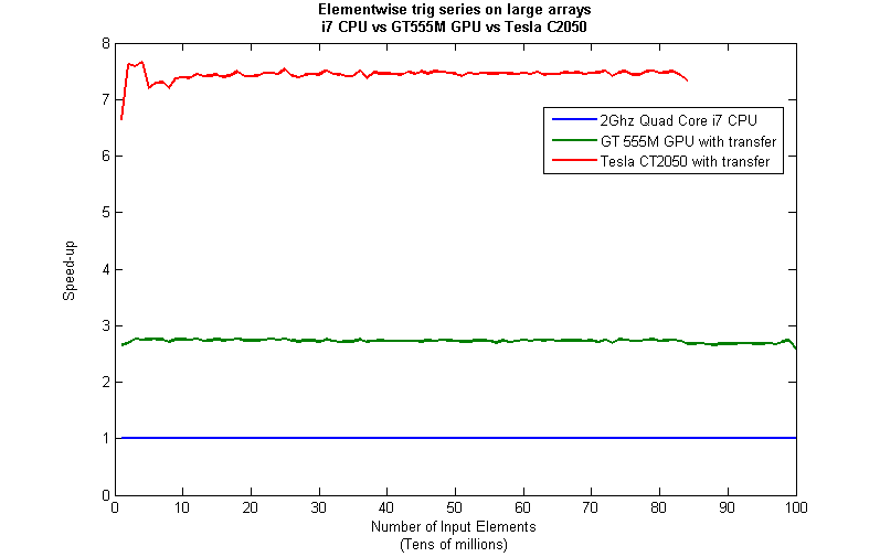
Just like last time, I ran this calculation on a range of input arrays from 1 million to 100 million elements on both my laptop’s GT 555M GPU and a Tesla C2050 I have access to.  Unfortunately, the C2050 is running MATLAB 2010b rather than 2011a so it’s not as fair a test as I’d like.  I could only get up to 84 million elements on the Tesla before it exited due to memory issues.  I’m not sure if this is down to the hardware itself or the fact that it was running an older version of MATLAB.

Next, I looked at the actual speed-up shown by the GPUs compared to my laptop’s i7 CPU.  Again, this includes data transfer times, is in full double precision and the CPU version was multi-threaded (No dodgy ‘GPUs are awesome’ techniques used here).  No matter what array size is used I get almost a factor of 3 speed-up using the laptop GPU and more than a factor of 7 speed-up when using the Tesla.  Not too shabby considering that the programming effort to achieve this speed-up was minimal.

Conclusions

• It is VERY easy to modify simple, element-wise functions to take advantage of the GPU in MATLAB using the Parallel Computing Toolbox.
• arrayfun is the most efficient way of dealing with such functions.
• My laptop’s GPU demonstrated almost a 3 times speed-up compared to its CPU.

Hardware / Software used for the majority of this article

• Laptop model: Dell XPS L702X
• CPU: Intel Core i7-2630QM @2Ghz software overclockable to 2.9Ghz. 4 physical cores but total 8 virtual cores due to Hyperthreading.
• GPU: GeForce GT 555M with 144 CUDA Cores.  Graphics clock: 590Mhz.  Processor Clock:1180 Mhz. 3072 Mb DDR3 Memeory
• RAM: 8 Gb
• OS: Windows 7 Home Premium 64 bit.  I’m not using Linux because of the lack of official support for Optimus.
• MATLAB: 2011a with the parallel computing toolbox

Code and sample timings (Will grow over time)

You need myseries.m and trigseries_test.m and the Parallel Computing Toolbox.  These are the times given by the following function call for various systems (transfer included and using arrayfun).

[cpu,~,~,~,gpu] = trigseries_test(10,50*1e6,'mean')

GPUs

• Tesla C2050, Linux, 2010b – 0.4751 seconds
• NVIDIA GT 555M – 144 CUDA Cores, 3Gb RAM, Windows 7, 2011a – 1.2986 seconds

CPUs

• Intel Core i7-2630QM, Windows 7, 2011a (My laptop’s CPU) – 3.33 seconds
• Intel Core 2 Quad Q9650 @ 3.00GHz, Linux, 2011a – 3.9452 seconds

Footnotes
1 – This is the method used in all subsequent timings and is similar to that used by the File Exchange function, timeit (timeit takes a median, I took a mean). If you prefer to use timeit then the function call would be timeit(@()myseries(cpu_x)). I stick to tic and toc in the article because it makes it clear exactly where timing starts and stops using syntax well known to most MATLABers.

Thanks to various people at The Mathworks for some useful discussions, advice and tutorials while creating this series of articles.

This lunchtime I stumbled across the following tweet by GrrlScientist

“mmm, cheese! RT @LookMaNoFans How many Calories would a Moon made of cheese be, you ask? A made-of-manchego Moon = 285 septillion Calories.”

A septillion is 10^24 so that’s a lot of calories!  Naturally, I wanted to check the facts so I asked Wolfram Alpha which, sadly, didn’t have the specifics on manchego cheese so I substituted monterey cheese to get a result of 8.5*10^25 calories. This disagrees with the tweet but it’s the figure I’m going to go with for now.

Since I am into running, I wondered how far I’d have to run to burn that many calories.  Using Wolfram Alpha’s running calorie calculator I found out that at a pace of 8 minutes per mile I would need to run 0.675 miles to burn 85 calories (assuming average body weight*) so would need to run 6.75*10^24 miles (almost 115 billion light years) to burn off the calories contained in a moon made of monteray cheese. That’s larger than the diameter of the observable universe!

*Obviously, if you ate the moon then you would weigh slightly more than average so this is a gross over-simplification.

Welcome to the heavily delayed 80th Carnival of Mathematics.  Apparently, 80 is the smallest number with exactly 7 representations as a sum of three distinct primes.  Head over to Wolfram Alpha to find them.  80 is also the smallest number that is diminished by taking its sum of letters (writing out its English name and adding the letters using a=1, b=2, c=3, …) – EIGHTY = 5+9+7+8+20+25 = 74 (Thanks Number Gossip).

Over at The Endeavour, John Cook discusses the principle of the single big jump (complete with SAGE notebooks) where he demonstrates that ‘your total progress is about as good as the progress on your best shot’…but only if the distribution is right.

Denise asks “What was it really like to work and think in Roman numerals, and then to suddenly learn the new way of calculating? Find out with these new books about math history.” in Fibonacci Puzzle.  She is also running a competition which will be ending very soon so you’ll need to hurry if you want to enter.

Guillermo Bautista discusses origami in Paper Folding: Locating the square root of a number on the number line while Gianluigi Filippelli explains how some researchers found a solution to a computational problem using a biological network.

David R. Wetzel gives us Saving the Sports Complex Algebra Project in an effort to better engage math students while Alexander Bogomolny brings us a whole host of engaging math activities for the summer break and Pat Ballew introduces a Sweet Geometry Challenge.

I came across a couple of interesting articles about Markov Chain Monte Carlo (MCMC) simulations this month.  The first is from John Cook, Markov Chains don’t converge while the second is by Danny Tarlow, Testing Intuitions about Markov Chain Monte Carlo: Do I have a bug?

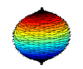
Matt Springer brings us Spherical Waves and the Hairy Ball Theorem (below)

Peter Rowlett of Travels in a Mathematical World fame recently had a paper published in Nature about the Unplanned Impact of Mathematics where he talks about how it can take decades, or even centuries, before research in pure mathematics can find applications in science and technology.  For example, quaternions, a 19th century discovery which seemed to have no practical value, have turned out to be invaluable to the 21st century computer games industry!  Something for the bean-counters to bear in mind when they obsess over short term impact factors of research.

Over at Futility Closet, we have a fun problem called School Reform.

Terence Tao gives us a geometric proof of the impossibility of angle trisection by straightedge and compass while the Geometry and the imagination blog discusses Rotation numbers and the Jankins-Neumann ziggurat.

Several people have been discussing recent changes in EPSRC (The UK’s main UK government agency for funding research and training in engineering and the physical sciences) including Timothy Gowers (A message from our sponsors), Burt Totaro (EPSRC dirigisme) and Paul Glendinning (Responding to EPSRC’s Shaping Capability Agenda).

Finally, one of my favourite mathematical websites is MathPuzzle.com.  Written by Ed Pegg Jr, it is possibly the best online resource for recreational mathematics you can find.  Go and take a look, you’ll be very glad you did.

That’s it for this month.  The next Carnival of Math will be over at Wild About Math on 2nd September and you can submit articles using the carnival submission form.  If you can’t wait until then, head over to I Hope This Old Train Breaks Down for the Math Teachers at Play carnival on August 19th.  If you are new to the math carnivals and are wondering what’s going on then take a look at my introduction to mathematics carnivals.

Follow the Carnival of Math on Twitter: @Carnivalofmath This is also the best way of reaching me if you’d like to be a future host for the carnival.