Walking Randomly

This is the first post on Walking Randomly that isn’t written by me!  I’ve been thinking about having guest writers on here for quite some time and when I first saw the tutorial below (written by Manchester University undergraduate, Gregory Astley) I knew that the time had finally come.  Greg is a student in Professor Bill Lionheart’s course entitled Asymptotic Expansions and Perturbation Methods where Mathematica is the software of choice.

Now, students at Manchester can use Mathematica on thousands of machines all over campus but we do not offer it for use on their personal machines.  So, when Greg decided to write up his lecture notes in Latex he needed to come up with an alternative way of producing all of the plots and he used the free, open source computer algebra system – Maxima.  I was very impressed with the quality of the plots that he produced and so I asked him if he would mind writing up a tutorial and he did so in fine style.  So, over to Greg….

This is a short tutorial on how to get up and running with the “plotdf” function for plotting direction fields/trajectories for 1st order autonomous ODEs in Maxima. My immediate disclaimer is that I am by no means an expert user!!! Furthermore, I apologise to those who have some experience with this program but I think the best way to proceed is to assume no prior knowledge of using this program or computer algebra systems in general.  Experienced users (surely more so than me) may feel free to skip the ‘boring’ parts.

Firstly, to those who may not know, this is a *free* (in both the “costs no money”, and “it’s open source” senses of the word) computer algebra system that is available to download on Windows, Mac OS, and Linux platforms from  http://maxima.sourceforge.net and it is well documented.

There are a number of different themes or GUIs that you can use with the program but I’ll assume we’re working with the somewhat basic “Xmaxima” shell.

Install and open up the program as you would do with any other and you will be greeted by the following screen.

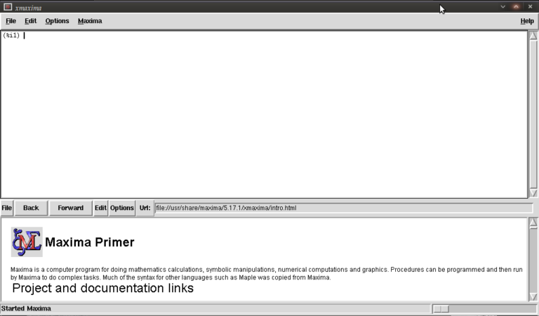
You are meant to type in the top most window next to (%i1) (input 1)
We first have to load the plotdf package (it isn’t loaded by default) so type:

load("plotdf");

and then press return (don’t forget the semi-colon or else nothing will happen (apart from a new line!)). it should respond with something similar to:

(%i1)  load("plotdf");
(%o1)  /usr/share/maxima/5.17.1/share/dynamics/plotdf.lisp
(%i2)

We will now race ahead and do our first plot. Keeping things simple for now we’ll do a phase plane plot for dx/dt = y, dy/dt = x, type:

plotdf([y,x]);

you should see something like this:

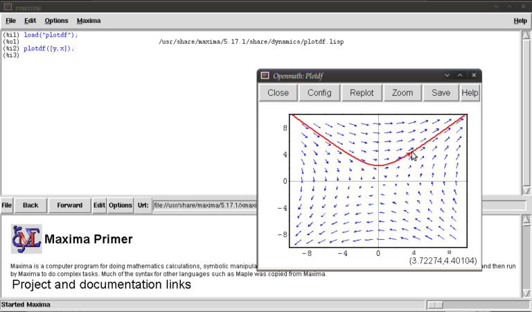
This is the Openmath plot window, (there are other plotting environments like Gnuplot but this function works only with Openmath) Notice that my pointer is directly below a red trajectory. These plots are interactive, you can draw other trajectories by clicking elsewhere. Try this.  Hit the “replot” button and it will redraw the direction field with just your last trajectory.

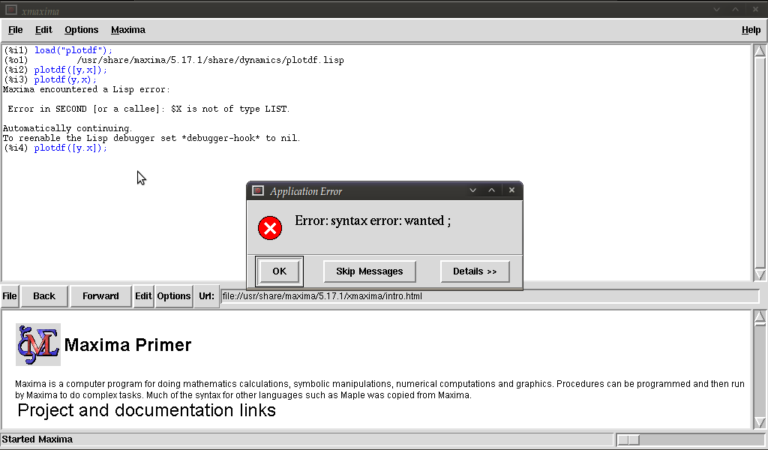
Before exploring any other options I want to purposely type some bad input and show how to fix things when it throws an error or gets stuck. Type

plotdf(y,x);

it should return

(%i3) plotdf(x,y);
Maxima encountered a Lisp error:

Error in SECOND [or a callee]: $Y is not of type LIST.

Automatically continuing.
To enable the Lisp debugger set *debugger-hook* to nil.
(%i4)

We forgot to put our functions for dx/dt,dy/dt in a list (square brackets). This is a reasonably safe error in that it tells us it isn’t happy and lets us continue.
Now type

plotdf([x.y]);

you should see something similar to

The problem this time was that we typed a dot instead of a comma (easily done), but worryingly when we close this message box and the blank plot the program will not process any commands. This can be fixed by clicking on the following in the xmaxima menu

file >> interrupt

where after telling you it encountered an error it should allow you to continue. One more; type

plotdf([2y,x]);

It should return with

  (%i5) plotdf([2y,x]);
  Incorrect syntax: Y is not an infix operator
  plotdf([2y,
           ^
  (%i5)

This time we forgot to put a binary operation such as * or + between 2 and y. If you come up with any other errors and the interrupt command is of no use you can still partially salvage things via

  file >> restart

but you will, in this case, have to load plotdf again. (mercifully you can go to the line where you first typed it and press return (as with other commands you might have done))
I will now demonstrate some more “contrived” plots (for absolutely no purpose other than to shamelessly give a (very) small gallery of standard functions/operations etc… for the novice user) there is no need to type the last four unless you want to see what happens by changing constants/parameters, they’re the same plot :)

  plotdf([2*y-%e^(3/2)+cos((%pi/2)*x),log(abs(x))-%i^2*y]);
  plotdf([integrate(2*y,y)/y,diff((1/2)*x^2,x)]);
  plotdf([(3/%pi)*acos(1/2)*y,(2/sqrt(%pi))*x*integrate(exp(-x^2),x,0,inf)]);
  plotdf([floor(1.43)*y,ceiling(.35)*x]);
  plotdf([imagpart(x+%i*y),(sum(x^n,n,0,2)-sum(x^j,j,0,1))/x]);

I could go on…notice that the constants pi, e, and i are preceded by “%”. This tells maxima that they are known constants as opposed to symbols you happened to call “pi”, “e”, and “i”. Also, noting that the default range for x and y is (-10,10) in both cases; feel free to replot the first of those five without wrapping x inside “abs()” (inside the logarithm that is). remember file >> interrupt afterwards!

Now I will introduce you to some more of the parameters you can plug into “plotdf(…)”. close any plot windows and type

plotdf([x,y],[x,1,5],[y,-5,5]);

You should notice that x now ranges from 1 to 5, whilst y ranges from -5 to 5. There is nothing special about these numbers, we could have chosen any *real* numbers we liked. You can also use different symbols for your variables instead of x or y. Try

plotdf([v,u],[u,v]);

Note that I’ve declared u and v as variables in the second list. I will now purposely do something wrong again. Assign the value 5 to x by typing

x:5;

then type

plotdf([y,x]);

This time maxima won’t throw an error because syntactically you haven’t done anything wrong, you merely told it to do

plotdf([y,5]);

as opposed to what you really wanted which is

plotdf([y,x]);

Surprisingly to me (discovered as I’m writing this), changing the names of your variables like we did above won’t save you since it seems to treat new symbols as merely placeholders for it’s favourite symbols x and y. To get round this type

kill(x);

and this will put x back to what it originally was (the symbol x as opposed to 5).
You don’t actually have to provide expressions for dx/dt and dy/dt, you might instead know dy/dx and you can generate phaseplots by typing say

plotdf([x/y]);

In this case we didn’t actually need the square brackets because we are providing only one parameter: dy/dx (x will be set to t by maxima giving dx/dt = 1, and dy/dt = dy/dx = x/y)

A number of parameters can be changed from within the openmath window. Type

plotdf([y,x],[trajectory_at,-1,-2],[direction,forward]);

and then go into config. The screen you get should look something like this:

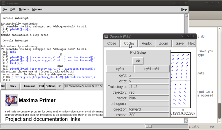
from here you can change the expressions for dx/dt, dy/dt, dy/dx, you can change colours and directions of trajectories (choices of forward, backward, both), change colours for direction arrows and orthogonal curves, starting points for trajectories (the two numbers separated by a space here, not a comma), time increments for t, number of steps used to create an integral curve. You can also look at an integral plots for x(t) and y(t) corresponding to the starting point given (or clicked) by hitting the “plot vs t” button. You can also zoom in or out by hitting the “zoom” button and clicking (or shift+clicking to unzoom), doing something else like hitting the config button will allow you to quit being in zoom mode click for trajectories again. (there might be a better way of doing this btw) You can also save these plots as eps files (you can then tweak these in other vector graphics based programs like Inkscape (free) or Adobe Illustrator etc..)

Interactive sliders

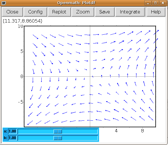
There are many permutations of things you can do (and you will surely find some of these by having a play) but my particular favourite is the option to use sliders allowing you to vary a parameter interactively and seeing what happens to the trajectories without constant replotting. ie:

plotdf([a*y,b*x],[sliders,"a=-1:3,b=-1:3"]);

Hopefully, this has been enough to get people started, and for what it’s worth, the help file (though using xmaxima, you’ll find this in the web-browser version) for this topic has a pretty good gallery of different plots and other parameters I didn’t mention.

just to throw in one last thing in the spirit of experimentation, is the following set of commands:

A:matrix([0,1],[1,0]);
B:matrix([x],[y]);
plotdf([A[1].B,A[2].B);

which is another way of doing the same old

plotdf([y,x]);

where here I’ve made a 2×2 matrix A, a 2×1 matrix B, with A[1], A[2] denoting rows 1 and 2 of A respectively and matrix multiplied the rows of A by B (using A[1].B, A[2].B) to serve as inputs for dx/dt and dy/dt

Tutorial written by Gregory Astley, Mathematics Undergraduate at The University of Manchester.

It’s been a great week for Open Source maths software this week with new releases of both Maxima and Scilab.

Maxima is a computer algebra system written in lisp that runs on most operating systems including Linux, Mac OS X and Windows.  The latest version, Maxima 5.20.1,  was released on Sunday 13th December and the full list of changes can be found here.  Highlights include improvements to the calculation of special functions, faster fourier transform routines and a general mechanism for functions to distribute over operators.

This last item is pretty cool since it allows you to map functions over lists in a similar manner to Mathematica.  For example, if you apply the sin function to a list in Maxima then you’ll now get a list containing the sines of each element of that list:

(%i1) sin([1,2,3]);
(%o1) [sin(1),sin(2),sin(3)]

Here are some examples of this new functionality for two-argument functions such as expintegral_e (taken from a post of Dieter Kaiser’s) include :

(%i2) expintegral_e([1,2,3],x);
(%o2) [expintegral_e(1,x),expintegral_e(2,x),expintegral_e(3,x)]

(%i3) expintegral_e(1,[x,y,z]);
(%o3) [expintegral_e(1,x),expintegral_e(1,y),expintegral_e(1,z)]

(%i4) expintegral_e([1,2,3],[x,y,z]);
(%o4) [[expintegral_e(1,x),expintegral_e(1,y),expintegral_e(1,z)],
       [expintegral_e(2,x),expintegral_e(2,y),expintegral_e(2,z)],
       [expintegral_e(3,x),expintegral_e(3,y),expintegral_e(3,z)]]

Head over to sourceforge to download Maxima for your operating system of choice. Now, onto Scilab….

Scilab is a fantastic open source numerical mathematics environment that always seems to come top of the list when people start discussing free MATLAB alternatives.  December 17th saw the release of Scilab 5.20 and the list of changes is epic (warning:pdf file).

The first new Scilab feature that caught my eye is the addition of a module called Xcos.  Xcos 1.0 is based on Scicos 4.3 which is a “graphical dynamical system modeler and simulator.”  Now I’ve not used any of this stuff before but as far as I can tell it could be considered as a free version of Simulink.  A bit of googling turned up a paper by M.G.J.M. Maassen, a student at the Eindoven University of Technology, who looked at the issue of migrating from Simulink to Scicos with respect to real time programs.  Written in 2006, this paper is slightly out of date but is a great start for anyone who is considering moving away from Simulink.

Along with other free mathematical software applications such as Octave, Sage, Python/Numpy and freemat, these new releases demonstrate that the world of free, open source mathematical applications has never looked better.