
Archive for the ‘Guest posts’ Category
This is a guest article written by friend, ex-colleague and keen user of Apple and Dropbox products, Ian Cottam of Manchester University’s IT Services.
Twice recently I have been bitten by being an early adopter of new software releases. Of course, I partly do this so colleagues at The University of Manchester don’t have to. Further, I have three Apple Macs and only update my least used one initially.
The two updates that bit me are: Mac OS X 10.11.0 El Capitan and the new Teams feature of Dropbox. My advice is not to use either of these updates (yet), unless you really need to. Interestingly, I persevered and have stayed with the Teams feature
of Dropbox; but have uninstalled OS X El Capitan by reverting to 10.10 Yosemite from a Time Machine backup.
Let’s do OS X El Capitan first.
This operating system update experience is the worst I can remember, and I have a long memory. What the legions of beta testers were doing I cannot imagine. To be fair, I expect many of them reported issues to Apple and just assumed Apple would not release to the public at large before they were fixed. I know I thought Apple would not release an OS that would kernel panic for many users on boot up. How wrong we all were.
A major, low-level change that Apple made for El Capitan was in the area of security; that is: kernel extensions, as used by some third party applications, have to be digitally signed to be acceptable. So far, so sensible. Some examples that I use include: VirtualBox, VMware, ncryptedCloud, github.osxfuse and Avatron. To see if you use any third party ones too, you can type the following into Terminal:
kextstat | grep -v com.apple
I expect over time all of the above will be updated to be digitally signed. However, at the time of writing some of them are not. Now quite why El Capitan does not log such unsigned extensions and ignore them on boot up I do not know. Instead you get a kernel panic and your Mac has become a brick. Well, not quite a brick as you can boot into safe mode (where extensions are not loaded) and try and fix things. But which ones are causing the problem? Not to mention that I would like to continue working with most, if not all, of them.
Googling shows that VirtualBox before version 5 and possibly nCrypted Cloud can ’cause’ the kernel panic; and I have several colleagues who persevered with updating to El Capitan by removing VirtualBox 4. I went back to Yosemite. (The fact that my Time Machine backup wasn’t as up to date as I would have liked is purely my fault. My other two Macs back up to Time Machine drives automatically, but my new Macbook waits for an external USB drive to be plugged in. I did try a restore from one of the other Time Machine drives that was 100% up to-date, but sadly the results were poor – e.g. the display driver – and I re-started the process from the specific but slightly out of date back-up.)
If you think that you can get around or live with this issue, I would further caution you to Google for Microsoft Office Problems El Capitan, to be further shocked. Ditto: Microsoft Outlook 2011 Problems El Capitan, if you are, like me, an Outlook/Exchange user.
I should repeat that some of my colleagues have updated to El Capitan and have not hit my problems or have worked around them.
Now on to Dropbox and its new Teams feature.
Teams is Dropbox’s way of bringing some of the advantages of Dropbox for Business to Dropbox Basic (the free version with quite limited storage) and Dropbox Pro (paid for, giving either 1TB or 2TB storage limits). Dropbox’s reason for doing this is so more people will update to Dropbox for Business (unlimited storage and greater admin control, etc.).
My first reason for being wary of Teams is that any member of a Team – not just the lead – can press the Update to Dropbox for Business button at anytime, committing and converting all in the Team. Now no doubt you can back out after a short trial period, but I expect it is a messy business (no pun intended).
What does the Teams feature offer? The first is to create a team or group list, such that when sharing appropriate folders you don’t need to list everyone in the team every time. Similarly, when a new team member starts, and once their email address is added to the group list, they will get copies of all all the existing shared folders. Good feature. I created a Team with just me in it for initial testing.
The other feature of Teams – the one I was most interested in – is the ability to have separate Work and Personal dropboxes under a single account on your Mac, PC or Linux box. If you are coming to Dropbox fresh, I would say go ahead and set up this feature, as it’s extremely handy to keep work and personal stuff completely separate. However, I had a mixture of work and private folders totalling some 120GB: that’s quite a bit to separate out. Now you face the decision as to whether the dropbox you currently have becomes your business one or your personal one. As I pay for Dropbox Pro myself I thought this fairly arbitrary and chose to keep my existing account as the business one. Your mileage may vary but I discovered I had more personal stuff in my dropbox than business, so the other way around might have saved me quite some time.
Your actual folder is renamed from “Dropbox” to “Dropbox (Your Choice of Business Name)”. As many folk have moaned about that, they also create a link to it with the old name of “Dropbox”. The next step is to set up, in my case, a new personal account (using a different email address) and link it to my main one. This is fairly straightforward. It’s also well done how easily you switch between your business and personal boxes. If like me, you have a 1TB account, that amount is shared between the two, although it is not obvious at first and you may get the odd message about the small size of your new dropbox, which you can safely ignore.
The thing that took a long time was copying all the personal stuff from what is now my business account to the personal one. You have to use the Dropbox desktop client for this. If a given sub-folder is not a share, you can try just dragging it over. I realised though that many of mine were shared. The only safe, if tedious, route I could find was to add my new personal identity to these shares; then transfer ownership – assuming I owned the share – and finally after the sync finished, remove my original identity from the share, unticking the box that says Keep a Copy. There might be an easier way: I hope so. I had a lot of shares to work through, and of course you are doing this on just one of the machines you own.
When done, I set up my second Mac, which was fairly straightforward and eventually everything synchronised to the right place. The big issue I had was with a third Mac that was further out of step. You guessed it: it was the one I had restored to Yosemite as mentioned in the first half of this blog. In such circumstances, Dropbox thinks you want to put lots of the folders back in to the original and now business identity. You can imagine how long that took and took me to unwind it back to how I had it with the two other Macs.
Perhaps I was both unlucky and made a bad choice or two, but be warned: for existing users with a complex dropbox setup this is rather painful to go through. I’m glad I did, but don’t find it easy to recommend to colleagues (yet).
Dropbox describe Teams here https://www.dropbox.com/help/9124.
Be careful out there, and don’t be an early adopter unless you are prepared for the pain.
This is a guest article written by friend and colleague, Ian Cottam. For part 1, see https://www.walkingrandomly.com/?p=5435
So why do computer scientists use (i != N) rather than the more common (i < N)?
When I said the former identifies “computer scientists” from others, I meant programmers who have been trained in the use of non-operational formal reasoning about their programs. It’s hard to describe that in a sentence or two, but it is the use of formal logic to construct-by-design and argue the correctness of programs or fragments of programs. It is non-operational because the meaning of a program fragment is derived (only) from the logical meaning of the statements of the programming language. Formal predicate logic is extended by extra rules that say what assignments, while loops, etc., mean in terms of logical proof rules for them.
A simple, and far from complete, example is what role the guard in a while/for loop condition in C takes.
for (i= 0; i != N; ++i) {
/* do stuff with a[i] */
}
without further thought (i.e. I just use the formal rule that says on loop termination the negation of the loop guard holds), I can now write:
for (i= 0; i != N; ++i) {
/* do stuff with a[i] */
}
/* Here: i == N */
which may well be key to reasoning that all N elements of the array have been processed (and no more). (As I said, lots of further formal details omitted.)
Consider the common form:
for (i= 0; i < N; ++i) {
/* do stuff with a[i] */
}
without further thought, I can now (only) assert:
for (i= 0; i < N; ++i) {
/* do stuff with a[i] */
}
/* Here: i >= N */
That is, I have to examine the loop to conclude the condition I really need in my reasoning: i==N.
Anyway, enough of logic! Let’s get operational again. Some programmers argue that i<N is more “robust” – in some, to me, strange sense – against errors. This belief is a nonsense and yet is widely held.
Let’s make a slip up in our code (for an example where the constant N is 9) in our initialisation of the loop variable i.
for (i= 10; i != N; ++i) {
/* do stuff with a[i] */
}
Clearly the body of my loop is entered, executed many many times and will quite likely crash the program. (In C we can’t really say what will happen as “undefined behaviour” means exactly that, but you get the picture.)
My program fragment breaks as close as possible to where I made the slip, greatly aiding me in finding it and making the fix required.
Now. . .the popular:
for (i= 10; i<N; ++i) {
/* do stuff with a[i]
}
Here, my slip up in starting i at 10 instead of 0 goes (locally) undetected, as the loop body is never executed. Millions of further statements might be executed before something goes wrong with the program. Worse, it may even not crash later but produce an answer you believe to be correct.
I find it fascinating that if you search the web for articles about this the i<N form is often strongly argued for on the grounds that it avoids a crash or undefined behaviour. Perhaps, like much of probability theory, this is one of those bits of programming theory that is far from intuitive.
Giants of programming theory, such as David Gries and Edsger Dijkstra, wrote all this up long ago. The most readable account (to me) came from Gries, building on Dijkstra’s work. I remember paying a lot of money for his book – The Science of Programming – back in 1981. It is now freely available online. See page 181 for his wording of the explanation above. The Science of Programming is an amazing book. It contains both challenging formal logic and also such pragmatic advice as “in languages that use the equal sign for assignment, use asymmetric layout to make such standout. In C we would write
var= expr;
rather than
var = expr; /* as most people again still do */
The visible signal I get from writing var= expr has stopped me from ever making the = for == mistake in C-like languages.
This is a guest article written by friend and colleague, Ian Cottam.
This brief guest piece for Walking Randomly was inspired by reading about some of the Hackday outputs at the recent SSI collaborative workshop CW14 held in Oxford. I wasn’t there, but I gather that some of the outputs from the day examined source code for various properties (perhaps a little tongue-in-cheek in some cases).
So, my also slightly tongue-in-cheek question is “Given a piece of source code written in a language with “while loops”: how do you know if the author is a computer scientist by education/training?”
I’ll use C as my language and note that “for loops” in C are basically syntactic sugar for while loops (allowing one to gather the initialisation, guard and increment parts neatly together). In other languages “for loops” are closer to Fortran’s original iterative “do loop”. Also, I will work with that subset of code fragments that obey traditional structured (one-entry, one-exit) programming constructs. If I didn’t, perhaps one could argue, as famously Dijkstra originally did, that the density of “goto” statements, even when spelt “break” or “continue”, etc., might be a deciding quality factor.
(Purely as an aside, I note that Linux (and related free/open source) contributors seem to use goto fairly freely as an exception case mechanism; and they might well have a justification. The density of gotos in Apple’s SSL code was illustrated recently by the so-called “goto fail” bug. See also Knuth’s famous article on this subject.)
In my own programming, I know from experience that if I use a goto, I find it so much more difficult to reason logically (and non-operationally) about my code that I avoid them. Whenever I have used a programming language without the goto statement, I have never missed it.
Now, finally to the point at hand, suppose one is processing the elements of an array of single dimension and of length N. The C convention is that the index goes from 0 to N-1. Code fragment A below is written by a non computer scientist, whereas B is.
/* Code fragment A */
for (i= 0; i < N; ++i) {

/* do stuff with a[i] */

}
/* Code fragment B */
for (i= 0; i != N; ++i) {

/* do stuff with a[i] */

}
The only difference is the loop’s guard: i<N versus i!=N.
As a computer scientist by training I would always write B; which would you write?
I would – and will in a follow-up – argue that B is better even though I am not saying that code fragment A is incorrect. Also in the follow-up I will acknowledge the computer scientist who first pointed this out – at least to me – some 33 years ago.
The Numerical Algorithms Group (NAG) are principally known for their numerical library but they also offer products such as a MATLAB toolbox and a Fortran compiler. My employer, The University of Manchester, has a full site license for most of NAG’s stuff where it is heavily used by both our students and researchers.
While at a recent software conference, I saw a talk by NAG’s David Sayers where he demonstrated some of the features of the NAG Fortran Compiler. During this talk he showed some examples of broken Fortran and asked us if we could spot how they were broken without compiler assistance. I enjoyed the talk and so asked David if he would mind writing a guest blog post on the subject for WalkingRandomly. He duly obliged.
This is a guest blog post by David Sayers of NAG.
What do you want from your Fortran compiler? Some people ask for extra (non-standard) features, others require very fast execution speed. The very latest extensions to the Fortran language appeal to those who like to be up to date with their code.
I suspect that very few would put enforcement of the Fortran standard at the top of their list, yet this essential if problems are to be avoided in the future. Code written specifically for one compiler is unlikely to work when computers change, or may contain errors that appear only intermittently. Without access to at least one good checking compiler, the developer or support desk will be lacking a valuable tool in the fight against faulty code.
The NAG Fortran compiler is such a tool. It is used extensively by NAG’s own staff to validate their library code and to answer user-support queries involving user’s Fortran programs. It is available on Windows, where it has its own IDE called Fortran Builder, and on Unix platforms and Mac OS X.
Windows users also have the benefit of some Fortran Tools bundled in to the IDE. Particularly nice is the Fortran polisher which tidies up the presentation of your source files according to user-specified preferences.
The compiler includes most Fortran 2003 features, very many Fortran 2008 features and the most commonly used features of OpenMP 3.0 are supported.
The principal developer of the compiler is Malcolm Cohen, co-author of the book, Modern Fortran Explained along with Michael Metcalf and John Reid. Malcolm has been a member of the international working group on Fortran, ISO/IEC JTC1/SC22/WG5, since 1988, and the USA technical subcommittee on Fortran, J3, since 1994. He has been head of the J3 /DATA subgroup since 1998 and was responsible for the design and development of the object-oriented features in Fortran 2003. Since 2005 he has been Project Editor for the ISO/IEC Fortran standard, which has continued its evolution with the publication of the Fortran 2008 standard in 2010.
Of all people Malcolm Cohen should know Fortran and the way the standard should be enforced!
His compiler reflects that knowledge and is designed to assist the programmer to detect how programs might be faulty due to a departure from the Fortran standard or prone to trigger a run time error. In either case the diagnostics of produced by the compiler are clear and helpful and can save the developer many hours of laborious bug-tracing. Here are some particularly simple examples of faulty programs. See if you can spot the mistakes, and think how difficult these might be to detect in programs that may be thousands of times longer:
Example 1
    Program test
      Real, Pointer :: x(:, :)

      Call make_dangle
      x(10, 10) = 0
    Contains
      Subroutine make_dangle
        Real, Target :: y(100, 200)

        x => y
      End Subroutine make_dangle
    End Program test
Example 2
Program dangle2
Real,Pointer :: x(:),y(:)
Allocate(x(100))
y => x
Deallocate(x)
y = 3
End
Example 3
      program more
      integer n, i
      real r, s
      equivalence (n,r)
      i=3
      r=2.5
      i=n*n
      write(6,900) i, r
900  format(' i = ', i5, '   r = ', f10.4)
      stop 'ok'
      end
Example 4
      program trouble1
      integer n
      parameter (n=11)
      integer iarray(n)
      integer i
      do 10 i=1,10
        iarray(i) = i
10   continue
      write(6,900) iarray
900  format(' iarray = ',11i5)
      stop 'ok'
      end
And finally if this is all too easy …
Example 5
!   E04UCA Example Program Text
!   Mark 23 Release. NAG Copyright 2011.

    MODULE e04ucae_mod

!      E04UCA Example Program Module:
!             Parameters and User-defined Routines

!      .. Use Statements ..
       USE nag_library, ONLY : nag_wp
!      .. Implicit None Statement ..
       IMPLICIT NONE
!      .. Parameters ..
       REAL (KIND=nag_wp), PARAMETER       :: one = 1.0_nag_wp
       REAL (KIND=nag_wp), PARAMETER       :: zero = 0.0_nag_wp
       INTEGER, PARAMETER                  :: inc1 = 1, lcwsav = 1,            &
                                              liwsav = 610, llwsav = 120,      &
                                              lrwsav = 475, nin = 5, nout = 6
    CONTAINS
       SUBROUTINE objfun(mode,n,x,objf,objgrd,nstate,iuser,ruser)
!         Routine to evaluate objective function and its 1st derivatives.

!         .. Implicit None Statement ..
          IMPLICIT NONE
!         .. Scalar Arguments ..
          REAL (KIND=nag_wp), INTENT (OUT)    :: objf
          INTEGER, INTENT (INOUT)             :: mode
          INTEGER, INTENT (IN)                :: n, nstate
!         .. Array Arguments ..
          REAL (KIND=nag_wp), INTENT (INOUT)  :: objgrd(n), ruser(*)
          REAL (KIND=nag_wp), INTENT (IN)     :: x(n)
          INTEGER, INTENT (INOUT)             :: iuser(*)
!         .. Executable Statements ..
          IF (mode==0 .OR. mode==2) THEN
             objf = x(1)*x(4)*(x(1)+x(2)+x(3)) + x(3)
          END IF

          IF (mode==1 .OR. mode==2) THEN
             objgrd(1) = x(4)*(x(1)+x(1)+x(2)+x(3))
             objgrd(2) = x(1)*x(4)
             objgrd(3) = x(1)*x(4) + one
             objgrd(4) = x(1)*(x(1)+x(2)+x(3))
          END IF

          RETURN

       END SUBROUTINE objfun
       SUBROUTINE confun(mode,ncnln,n,ldcj,needc,x,c,cjac,nstate,iuser,ruser)
!         Routine to evaluate the nonlinear constraints and their 1st
!         derivatives.

!         .. Implicit None Statement ..
          IMPLICIT NONE
!         .. Scalar Arguments ..
          INTEGER, INTENT (IN)                :: ldcj, n, ncnln, nstate
          INTEGER, INTENT (INOUT)             :: mode
!         .. Array Arguments ..
          REAL (KIND=nag_wp), INTENT (OUT)    :: c(ncnln)
          REAL (KIND=nag_wp), INTENT (INOUT)  :: cjac(ldcj,n), ruser(*)
          REAL (KIND=nag_wp), INTENT (IN)     :: x(n)
          INTEGER, INTENT (INOUT)             :: iuser(*)
          INTEGER, INTENT (IN)                :: needc(ncnln)
!         .. Executable Statements ..
          IF (nstate==1) THEN

!            First call to CONFUN.  Set all Jacobian elements to zero.
!            Note that this will only work when 'Derivative Level = 3'
!            (the default; see Section 11.2).

             cjac(1:ncnln,1:n) = zero
          END IF

          IF (needc(1)>0) THEN

             IF (mode==0 .OR. mode==2) THEN
                c(1) = x(1)**2 + x(2)**2 + x(3)**2 + x(4)**2
             END IF

             IF (mode==1 .OR. mode==2) THEN
                cjac(1,1) = x(1) + x(1)
                cjac(1,2) = x(2) + x(2)
                cjac(1,3) = x(3) + x(3)
                cjac(1,4) = x(4) + x(4)
             END IF

          END IF

          IF (needc(2)>0) THEN

             IF (mode==0 .OR. mode==2) THEN
                c(2) = x(1)*x(2)*x(3)*x(4)
             END IF

             IF (mode==1 .OR. mode==2) THEN
                cjac(2,1) = x(2)*x(3)*x(4)
                cjac(2,2) = x(1)*x(3)*x(4)
                cjac(2,3) = x(1)*x(2)*x(4)
                cjac(2,4) = x(1)*x(2)*x(3)
             END IF

          END IF

          RETURN

       END SUBROUTINE confun
    END MODULE e04ucae_mod
    PROGRAM e04ucae

!      E04UCA Example Main Program

!      .. Use Statements ..
       USE nag_library, ONLY : dgemv, e04uca, e04wbf, nag_wp
       USE e04ucae_mod, ONLY : confun, inc1, lcwsav, liwsav, llwsav, lrwsav,   &
                               nin, nout, objfun, one, zero
!      .. Implicit None Statement ..
!       IMPLICIT NONE
!      .. Local Scalars ..
      ! REAL (KIND=nag_wp)                  :: objf
       INTEGER                             :: i, ifail, iter, j, lda, ldcj,    &
                                              ldr, liwork, lwork, n, nclin,    &
                                              ncnln, sda, sdcjac
!      .. Local Arrays ..
       REAL (KIND=nag_wp), ALLOCATABLE     :: a(:,:), bl(:), bu(:), c(:),      &
                                              cjac(:,:), clamda(:), objgrd(:), &
                                              r(:,:), work(:), x(:)
       REAL (KIND=nag_wp)                  :: ruser(1), rwsav(lrwsav)
       INTEGER, ALLOCATABLE                :: istate(:), iwork(:)
       INTEGER                             :: iuser(1), iwsav(liwsav)
       LOGICAL                             :: lwsav(llwsav)
       CHARACTER (80)                      :: cwsav(lcwsav)
!      .. Intrinsic Functions ..
       INTRINSIC                              max
!      .. Executable Statements ..
       WRITE (nout,*) 'E04UCA Example Program Results'

!      Skip heading in data file
       READ (nin,*)

       READ (nin,*) n, nclin, ncnln
       liwork = 3*n + nclin + 2*ncnln
       lda = max(1,nclin)

       IF (nclin>0) THEN
          sda = n
       ELSE
          sda = 1
       END IF

       ldcj = max(1,ncnln)

       IF (ncnln>0) THEN
          sdcjac = n
       ELSE
          sdcjac = 1
       END IF

       ldr = n

       IF (ncnln==0 .AND. nclin>0) THEN
          lwork = 2*n**2 + 20*n + 11*nclin
       ELSE IF (ncnln>0 .AND. nclin>=0) THEN
          lwork = 2*n**2 + n*nclin + 2*n*ncnln + 20*n + 11*nclin + 21*ncnln
       ELSE
          lwork = 20*n
       END IF

       ALLOCATE (istate(n+nclin+ncnln),iwork(liwork),a(lda,sda), &
          bl(n+nclin+ncnln),bu(n+nclin+ncnln),c(max(1, &
          ncnln)),cjac(ldcj,sdcjac),clamda(n+nclin+ncnln),objgrd(n),r(ldr,n), &
          x(n),work(lwork))

       IF (nclin>0) THEN
          READ (nin,*) (a(i,1:sda),i=1,nclin)
       END IF

       READ (nin,*) bl(1:(n+nclin+ncnln))
       READ (nin,*) bu(1:(n+nclin+ncnln))
       READ (nin,*) x(1:n)

!      Initialise E04UCA

       ifail = 0
       CALL e04wbf('E04UCA',cwsav,lcwsav,lwsav,llwsav,iwsav,liwsav,rwsav, &
          lrwsav,ifail)

!      Solve the problem

       ifail = -1
       CALL e04uca(n,nclin,ncnln,lda,ldcj,ldr,a,bl,bu,confun,objfun,iter, &
          istate,c,cjac,clamda,objf,objgrd,r,x,iwork,liwork,work,lwork,iuser, &
          ruser,lwsav,iwsav,rwsav,ifail)

       SELECT CASE (ifail)
       CASE (0:6,8)
          WRITE (nout,*)
          WRITE (nout,99999)
          WRITE (nout,*)

          DO i = 1, n
             WRITE (nout,99998) i, istate(i), x(i), clamda(i)
          END DO

          IF (nclin>0) THEN

!            A*x --> work.
!            The NAG name equivalent of dgemv is f06paf
             CALL dgemv('N',nclin,n,one,a,lda,x,inc1,zero,work,inc1)

             WRITE (nout,*)
             WRITE (nout,*)
             WRITE (nout,99997)
             WRITE (nout,*)

             DO i = n + 1, n + nclin
                j = i - n
                WRITE (nout,99996) j, istate(i), work(j), clamda(i)
             END DO

          END IF

          IF (ncnln>0) THEN
             WRITE (nout,*)
             WRITE (nout,*)
             WRITE (nout,99995)
             WRITE (nout,*)

             DO i = n + nclin + 1, n + nclin + ncnln
                j = i - n - nclin
                WRITE (nout,99994) j, istate(i), c(j), clamda(i)
             END DO

          END IF

          WRITE (nout,*)
          WRITE (nout,*)
          WRITE (nout,99993) objf
       END SELECT

99999  FORMAT (1X,'Varbl',2X,'Istate',3X,'Value',9X,'Lagr Mult')
99998  FORMAT (1X,'V',2(1X,I3),4X,1P,G14.6,2X,1P,G12.4)
99997  FORMAT (1X,'L Con',2X,'Istate',3X,'Value',9X,'Lagr Mult')
99996  FORMAT (1X,'L',2(1X,I3),4X,1P,G14.6,2X,1P,G12.4)
99995  FORMAT (1X,'N Con',2X,'Istate',3X,'Value',9X,'Lagr Mult')
99994  FORMAT (1X,'N',2(1X,I3),4X,1P,G14.6,2X,1P,G12.4)
99993  FORMAT (1X,'Final objective value = ',1P,G15.7)
    END PROGRAM e04ucae
Answers to this particular New Year quiz will be posted in a future blog post.
This is a guest post by colleague and friend, Ian Cottam of The University of Manchester.
I recently implemented a lint program for Condor (unsurprisingly called: condor_lint), analogous to the famous one for C of days of yore. That is, it points out the fluff in a Condor script and suggests improvements. It is based on our local knowledge of how our Condor Pool is set up, here in Manchester, and also reflects recent changes to Condor.
Why I did it is interesting and may have wider applicability. Everything it reports is already written up on our extensive internal web site which users rarely read. I suspect the usual modus operandi of our users is to find, or be given, a Condor script, relevant to their domain, and make the minimum modifications to it that means it ‘works’. Subsequently, its basic structure is never updated (apart from referencing new data files, etc).
To be fair, that’s what we all do — is it not?
Ignoring our continually updated documentation means that a user’s job may make poor use of the Condor Pool, affecting others, and costing real money (in wasted energy) through such “bad throughput”.
Now, although we always run the user’s job if Condor’s basic condor_submit command accepts it, we first automatically run condor_lint. This directly tells them any “bad news” and also, in many cases, gives them the link to the specific web page that explains the issue in detail.
Clearly, even such “in your face” advice can still be ignored, but we are starting to see improvements.
Obviously such an approach is not limited to Condor, and we would be interested in hearing of “lint approaches” with other systems.
Links
Other WalkingRandomly posts by Ian Cottam
A guest post by Ian Cottam (@iandavidcottam).
I have been a programmer for 40 years this month. I thought I would write a short essay on things I experienced over that time that went into the design of a relatively recent, small program: DropAndCompute. (The purpose and general evolution of that program were described in a blog entry here. Please just watch the video there if you are new to DropAndCompute.)
Once I had the idea for DropAndCompute –inspired equally by the complexity of Condor and the simplicity of Dropbox — I coded and tested it in about two days. (Typically, one bug lasted until it had a real user, but it was no big deal.) My colleague, Mark Whidby, later re-factored/re-coded it to better scale as it grew in popularity here at The University of Manchester. I expect Mark spent about two days on it too. The user interface and basic design did not change. (As the evolution blog discusses, we eventually made the use of Dropbox optional, but that does not detract from this tale.)
Physically dropping programs and their data:
In the early to mid 1970s as well as doing my own programming work I helped scientists in Liverpool to run their code. One approach we used to make them faster was to drop the deck of cards into the input well of a card reader which was remotely connected to the regional supercomputer centre at Manchester. (I never knew what the communication mechanism was – probably a wet string given the technology of the time.) A nearby line printer was similarly connected and our results could be picked up, usually the next day. DropAndCompute is a 21st century version of this activity, without the leg work and humping of large boxes of cards about.
That this approach was worth the effort was made obvious with one of the first card decks I ever submitted. We had been running the code on an ICL 1903A computer in Liverpool; Manchester had a CDC 6600 (hopefully my memory has not let me down – it did become a CDC 7600 at some stage). Running the code locally in Liverpool, with typical data, took around 55 CPU minutes. Dropping it into that card reader so that it automatically ran in Manchester resulted in the jaw dropping time of 4 CPU seconds. (I still had to wait overnight to pick up the results, something that resonates with today’s DropAndCompute users and Manchester’s Condor Pool, which is only large and powerful overnight.)
Capabilities:
Later, but still in the mid 1970s, I worked for Plessey on their System 250 high-reliability, multiprocessor system. It was the first commercial example of a capability architecture. With such there is no supervisor state or privileged code rings or similar. If you held the capability to do something (e.g. read, write or enter another code context) you could do it. If you didn’t hold the appropriate capability, you could not. The only tiny section of code in the System 250 that was special was where capabilities were generated. No one else could make them.
The server side of DropAndCompute generates capabilities to the user client side. They are implemented as zero length files whose information content is just in their names. For job 3159, you get 3159.kill, 3159.vacate and 3159.debug generated*. By dragging and dropping one or more of these zero length files (capabilities) onto the dropbox the remote lower level Condor command code is automatically executed. [* You could try to make your own capability, such as 9513.kill, but it won’t work.]
UNIX and Shell Glue Code:
My initial exposure to the UNIX tools philosophy in the late 1970s profoundly influenced me (and still does). In essence, it says that one should build new software by inventing ‘glue’ to stick existing components together. The UNIX Shell is often the language of choice for this, and was for me. DropAndCompute is a good example of where a little bit of glue produced a hopefully impressive synergy.
The Internet not The Web:
DropAndCompute uses the Internet (clearly). It is not a Web application. I only mention this as some younger programmers, who have grown up with the Web always being there, seem to think the best/only architecture to use for a software system design is one implemented through a web browser using web services. I am grateful to be able to remember pre-Web days, as much as I love what Tim Berners-Lee created for us.
Client-Server:
I’m not sure when I first became aware of client-server architecture. I know a famous computer scientist (the late David Wheeler*) once described it as simply the obvious way to implement software systems. For my part, I’m a believer in the less code the client side (user) needs to install the better (less to go wrong on strange environments one has no control over). In the case of DropAndCompute if the user had Dropbox, it was nothing to install, and just downloading Dropbox if they didn’t.
[* As well as being a co-inventer of the subroutine, David Wheeler led the team that designed the first operational capability-based computer: the Cambridge University CAP.]
Rosetta – Software as Magic:
Around a decade ago I worked for Transitive, a University of Manchester spin-out, and the company that produced Rosetta for Apple. With apologies to Arthur C Clarke: all great software appears to be magic to the user. The simpler the user interface, often the more complex the underlying system is to implement the magic. This is true, for example, for Apple iOS and OS X and for Dropbox (simpler, and yet I would bet that it is internally more complex, than its many competitors). One small part of OS X I helped with is Rosetta (or was, as Apple dropped it from the Lion 10.7 release of OS X). Rosetta dynamically (i.e. on-the-fly) translates PowerPC applications into Intel x86 code. There is no noticeable user interface: you double click your desired application, like any other, and, if needed, Rosetta is invoked to do its job in the background.
I have read many interesting web based discussions about Rosetta, several say, or imply, that it is a relatively simple piece of software: nothing could be further from the truth. It’s likely still a commercial secret how it works, but if it were simple, Apple’s transition to Intel would likely have been a disaster. It took a lot of smart people a long time to make the magic appear that simple.
I tried to keep DropAndCompute’s interface to the user as simple as possible, even where it added some complexity to its implementation. The National Grid Service in the UK did their own version of DropAndCompute, but, for my taste, added too many bells and whistles.
In Conclusion:
I hope this brief essay has been of interest and given some insight into how many years of software/system design experience come to be applied, even to small software systems, both consciously and subconsciously, and always, hopefully, with good taste. Hide complexity, keep it simple for the user, make them think it is simply magic!
A couple of weeks ago my friend and colleague, Ian Cottam, wrote a guest post here at Walking Randomly about his work on interfacing Dropbox with the high throughput computing software, Condor. Ian’s post was very well received and so he’s back; this time writing about a very different kind of project. Over to Ian.
Natural Scientists: their very big output files – and a tale of diffs by Ian Cottam
I’ve noticed that natural scientists (as opposed to computer scientists) often write, or use, programs that produce masses of output, usually just numbers. It might be the final results file or, often, some intermediate test results.
Am I being a little cynical in thinking that many users glance – ok, carefully check – a few of these thousands (millions?) of numbers and then delete the file? Let’s assume such files are really needed. A little automation is often added to the process by having a baseline file and running a program to show you the differences between it and your latest output (assuming wholesale changes are not the norm).
One of the popular difference programs is the Unix diff command . (I’ve been using it since the 1970s.) It popularised the idea of showing minimal differences between two text files (and, later, binary ones too). There are actually a few algorithms for doing minimal difference computation, and GNU diff, for example, uses a different one from the original Bell Labs version. They all have one thing in common: to achieve minimal difference computation the two files being compared must be read into main memory (aka RAM). Back in the 1970s, and on my then department’s PDP-11/40, this restricted the size of the files considerably; not that we noticed much as everything was 16bit and “small was beautiful”. GNU diff, on modern machines, can cope with very big files, but still chokes if your files, in aggregate, approach the gigabyte range.
(As a bit of an aside: a major contribution of all the GNU tools, over what we had been used to from the Unix pioneers at Bell Labs, was that they removed all arbitrary size restrictions; the most common and frustrating one being the length of text lines.)
Back to the 1970s again: Bell Labs did know that some files were too big to compare with diff , and they also shipped: diffh. The h stands for halfhearted. Diffh does not promise minimal differences, but can be very good for big files with occasional differences. It uses a pass over the files using a simple ‘sliding window’ heuristic approach (the other word that the h is sometimes said to stand for). You can still find an old version of diffh on the Internet. However, it ‘gives up’ rather easily and you may have to spend some time modifying it for, e.g., 64 bit ints and pointers, as well as for compiling with modern C compilers. Other tools exist that can compare enormous files, but they don’t produce readable output in diff’s pleasant format.
A few years back, when a user at the University of Manchester asked for help with the ‘diff – files too big/ out of memory’ problem, I wrote a modern version that I called idiffh (for Ian’s diffh). My ground rules were:
- Work on any text files on any operating system with a C compiler
- Have no limits on, e.g., line lengths or file size
- Never ‘give up’ if the going gets tough (i.e. when the files are very different)
You won’t find this with the GNU collection as they like to write code to the Unix interface and I like to write to the C standard I/O interface (see the first bullet point above).
An interesting implementation detail is that it uses random access to the files directly, relying on the operating system’s cache of file blocks to make this tolerably efficient. Waiting a minute or two to compare gigabyte sized files is usually acceptable.
As the comments in the code say, you can get some improvements by conditional compilation on Unix systems and especially on BSD Systems (including Apple Macs), but you can compile it straight, without such, on Windows and other platforms.
If you would like to try idffh out you can download it here.
In my previous blog post I mentioned that I am a member of a team that supports High Throughput Computing (HTC) at The University of Manchester via a 1600+ core ‘condor pool’. In order to make it as easy as possible for our researchers to make use of this resource one of my colleagues, Ian Cottam, created a system called DropAndCompute. In this guest blog post, Ian describes DropAndCompute and how it evolved into the system we use at Manchester today.
The Evolution of “DropAndCompute” by Ian Cottam
DropAndCompute, as used at The University of Manchester’s Faculty of Engineering and Physical Sciences, is an approach to using network (or grid or cloud based) computational resources without having to know the operating system of the resource’s gateway or any command line tools of either the resource itself —Condor in our case — or in general. Most such gateways run a flavour of Unix, often Linux. Many of our users are either unfamiliar with Linux or just prefer a drag-and-drop interface, as I do myself despite using various flavours of Unix since Version 6 in the late 70s.
Why did I invent it? On its original web site description page wiki.myexperiment.org/index.php/DropAndCompute the following reasons are given:
- A simple and uniform drag-and-drop graphical user interface, potentially, to many resource pools.
- No use of terminal windows or command lines.
- No need to login to remote hosts or install complicated grid-enabling software locally.
- No need for the user to have an account on the remote resources (instead they are accounted by having a shared folder allocated). Of course, nothing stops the users from having accounts should that be preferred.
- No need for complicated Virtual Private Networks, IP Tunnelling, connection brokers, or similar, in order to access grid resources on private subnets (provided at least one node is on the public Internet, which is the norm).
- Pop-ups notify users of important events (basically, log and output files being created when a job has been accepted, and when the generated result files arrive).
- Somewhat increased security as the user only has (indirect) access to a small subset of the computational resource’s commands.
Version One
The first version was used on a Condor Pool within our interdisciplinary biocentre (MIB). A video of it in use is shown below
Please do take the time to look at this video as it shows clearly how, for example, Condor can be used via this type of interface.
This version was notable for using the commercial service: Dropbox and, in fact, my being a Dropbox user inspired the approach and its name. Dropbox is trivial to install on any of the main platforms, on any number of computers owned by a user, and has a free version giving 2GB of synchronised and shared storage. In theory, only the computational resource supplier need pay for a 100GB account with Dropbox, have a local Condor submitting account, and share folders out with users of the free Dropbox-based service.
David De Roure, then at the University of Southampton and now Oxford, reviewed this approach here at blog.openwetware.org/deroure/?p=97, and offers his view as to why it is important in helping scientists start on the ‘ramp’ to using what can be daunting, if powerful, computational facilities.
Version Two
Quickly the approach migrated to our full, faculty-wide Condor Pool and the first modification was made. Now we used separate accounts for each user of the service on our submitting nodes; Dropbox still made this sharing scheme trivial to set up and manage, whilst giving us much better usage accounting information. The first minor problem came when some users needed more –much more in fact– than 2GB of space. This was solved by them purchasing their own 50GB or 100GB accounts from Dropbox.
Problems and objections
However, two more serious problems impacted our Dropbox based approach. First, the large volume of network traffic across the world to Dropbox’s USA based servers and then back down to local machines here in Manchester resulted in severe bottlenecks once our Condor Pool had reached the dizzy heights of over a thousand processor cores. We could have ameliorated this by extra resources, such as multiple submit nodes, but the second problem proved to be more of a showstopper.
Since the introduction of DropAndCompute several people –at Manchester and beyond– have been concerned about research data passing through commercial, USA-based servers. In fact, the UK’s National Grid Service (NGS) who have implemented their own flavour of DropAndCompute did not use Dropbox for this very reason. The US Patriot Act means that US companies must surrender any data they hold if officially requested to do so by Federal Government agencies. Now one approach to this is to do user-level encryption of the data before it enters the user’s dropbox. I have demonstrated this approach, but it complicates the model and it is not so straightforward to use exactly the same method on all of the popular platforms (Windows, Mac, Linux).
Version Three
To tackle the above issues we implemented a ‘local version’ of DropAndCompute that is not Dropbox based. It is similar to the NGS approach, but, in my opinion, much simpler to setup. The user merely has to mount a folder on the submit node on their local computer(s), and then use the same drag-and-drop approach to get the job initiated, debugged and run (or even killed, when necessary). This solves the above issues, but could be regarded as inferior to the Dropbox based approach in five ways:
1. The convenience and transparency of ‘offline’ use. That is, Dropbox jobs can be prepared on, say, a laptop with or without net access, and when the laptop next connects the job submissions just happens. Ditto for the results coming back.
2. When online and submitting or waiting for results with the local version, the folder windows do not update to give the user an indication of progress.
3. Users must remember to use an email notification that a job has finished, or poll to check its status.
4. The initial setup is a little harder for the local version compared with using Dropbox.
5. The computation’s result files are not copied back automatically.
So far, only item 5 has been remarked on by some of our users, and it, and the others, could be improved with some programming effort.
A movie of this version is shown below; it doesn’t have any commentary, but essentially follows the same steps as the Dropbox based video. You will see the network folder’s window having to be refreshed manually –this is necessary on a Mac (but could be scripted); other platforms may be better– and results having to be dragged back from the mounted folder.
I welcome comments on any aspect of this –still evolving– approach to easing the entry ‘cost’ to using distributed computing resources.
Acknowledgments
Our Condor Pool is supported by three colleagues besides myself: Mark Whidby, Mike Croucher and Chris Paul. Mark, inter alia, maintains the current version of DropAndCompute that can operate locally or via Dropbox. Thanks also to Mike for letting me be a guest on Walking Randomly.
This is the first post on Walking Randomly that isn’t written by me! I’ve been thinking about having guest writers on here for quite some time and when I first saw the tutorial below (written by Manchester University undergraduate, Gregory Astley) I knew that the time had finally come. Greg is a student in Professor Bill Lionheart’s course entitled Asymptotic Expansions and Perturbation Methods where Mathematica is the software of choice.
Now, students at Manchester can use Mathematica on thousands of machines all over campus but we do not offer it for use on their personal machines. So, when Greg decided to write up his lecture notes in Latex he needed to come up with an alternative way of producing all of the plots and he used the free, open source computer algebra system – Maxima. I was very impressed with the quality of the plots that he produced and so I asked him if he would mind writing up a tutorial and he did so in fine style. So, over to Greg….
This is a short tutorial on how to get up and running with the “plotdf” function for plotting direction fields/trajectories for 1st order autonomous ODEs in Maxima. My immediate disclaimer is that I am by no means an expert user!!! Furthermore, I apologise to those who have some experience with this program but I think the best way to proceed is to assume no prior knowledge of using this program or computer algebra systems in general. Experienced users (surely more so than me) may feel free to skip the ‘boring’ parts.
Firstly, to those who may not know, this is a *free* (in both the “costs no money”, and “it’s open source” senses of the word) computer algebra system that is available to download on Windows, Mac OS, and Linux platforms from http://maxima.sourceforge.net and it is well documented.
There are a number of different themes or GUIs that you can use with the program but I’ll assume we’re working with the somewhat basic “Xmaxima” shell.
Install and open up the program as you would do with any other and you will be greeted by the following screen.
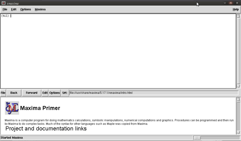
You are meant to type in the top most window next to (%i1) (input 1)
We first have to load the plotdf package (it isn’t loaded by default) so type:
load("plotdf");
and then press return (don’t forget the semi-colon or else nothing will happen (apart from a new line!)). it should respond with something similar to:
(%i1)  load("plotdf");
(%o1)  /usr/share/maxima/5.17.1/share/dynamics/plotdf.lisp
(%i2)
We will now race ahead and do our first plot. Keeping things simple for now we’ll do a phase plane plot for dx/dt = y, dy/dt = x, type:
plotdf([y,x]);
you should see something like this:
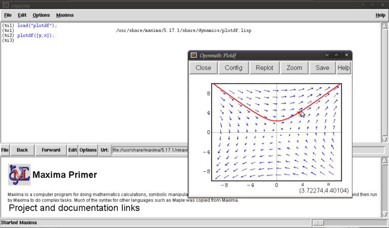
This is the Openmath plot window, (there are other plotting environments like Gnuplot but this function works only with Openmath) Notice that my pointer is directly below a red trajectory. These plots are interactive, you can draw other trajectories by clicking elsewhere. Try this. Hit the “replot” button and it will redraw the direction field with just your last trajectory.
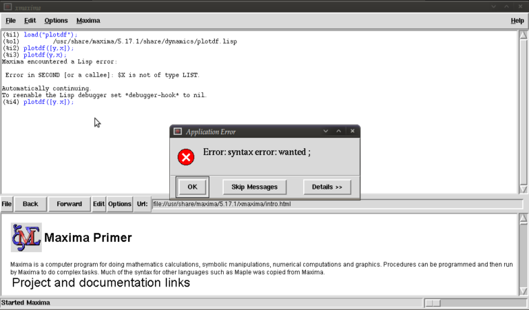
Before exploring any other options I want to purposely type some bad input and show how to fix things when it throws an error or gets stuck. Type
plotdf(y,x);
it should return
(%i3) plotdf(x,y);
Maxima encountered a Lisp error:

Error in SECOND [or a callee]: $Y is not of type LIST.

Automatically continuing.
To enable the Lisp debugger set *debugger-hook* to nil.
(%i4)
We forgot to put our functions for dx/dt,dy/dt in a list (square brackets). This is a reasonably safe error in that it tells us it isn’t happy and lets us continue.
Now type
plotdf([x.y]);
you should see something similar to
The problem this time was that we typed a dot instead of a comma (easily done), but worryingly when we close this message box and the blank plot the program will not process any commands. This can be fixed by clicking on the following in the xmaxima menu
file >> interrupt
where after telling you it encountered an error it should allow you to continue. One more; type
plotdf([2y,x]);
It should return with
  (%i5) plotdf([2y,x]);
  Incorrect syntax: Y is not an infix operator
  plotdf([2y,
           ^
  (%i5)
This time we forgot to put a binary operation such as * or + between 2 and y. If you come up with any other errors and the interrupt command is of no use you can still partially salvage things via
file >> restart
but you will, in this case, have to load plotdf again. (mercifully you can go to the line where you first typed it and press return (as with other commands you might have done))
I will now demonstrate some more “contrived” plots (for absolutely no purpose other than to shamelessly give a (very) small gallery of standard functions/operations etc… for the novice user) there is no need to type the last four unless you want to see what happens by changing constants/parameters, they’re the same plot :)
  plotdf([2*y-%e^(3/2)+cos((%pi/2)*x),log(abs(x))-%i^2*y]);
  plotdf([integrate(2*y,y)/y,diff((1/2)*x^2,x)]);
  plotdf([(3/%pi)*acos(1/2)*y,(2/sqrt(%pi))*x*integrate(exp(-x^2),x,0,inf)]);
  plotdf([floor(1.43)*y,ceiling(.35)*x]);
  plotdf([imagpart(x+%i*y),(sum(x^n,n,0,2)-sum(x^j,j,0,1))/x]);
I could go on…notice that the constants pi, e, and i are preceded by “%”. This tells maxima that they are known constants as opposed to symbols you happened to call “pi”, “e”, and “i”. Also, noting that the default range for x and y is (-10,10) in both cases; feel free to replot the first of those five without wrapping x inside “abs()” (inside the logarithm that is). remember file >> interrupt afterwards!
Now I will introduce you to some more of the parameters you can plug into “plotdf(…)”. close any plot windows and type
plotdf([x,y],[x,1,5],[y,-5,5]);
You should notice that x now ranges from 1 to 5, whilst y ranges from -5 to 5. There is nothing special about these numbers, we could have chosen any *real* numbers we liked. You can also use different symbols for your variables instead of x or y. Try
plotdf([v,u],[u,v]);
Note that I’ve declared u and v as variables in the second list. I will now purposely do something wrong again. Assign the value 5 to x by typing
x:5;
then type
plotdf([y,x]);
This time maxima won’t throw an error because syntactically you haven’t done anything wrong, you merely told it to do
plotdf([y,5]);
as opposed to what you really wanted which is
plotdf([y,x]);
Surprisingly to me (discovered as I’m writing this), changing the names of your variables like we did above won’t save you since it seems to treat new symbols as merely placeholders for it’s favourite symbols x and y. To get round this type
kill(x);
and this will put x back to what it originally was (the symbol x as opposed to 5).
You don’t actually have to provide expressions for dx/dt and dy/dt, you might instead know dy/dx and you can generate phaseplots by typing say
plotdf([x/y]);
In this case we didn’t actually need the square brackets because we are providing only one parameter: dy/dx (x will be set to t by maxima giving dx/dt = 1, and dy/dt = dy/dx = x/y)
A number of parameters can be changed from within the openmath window. Type
plotdf([y,x],[trajectory_at,-1,-2],[direction,forward]);
and then go into config. The screen you get should look something like this:
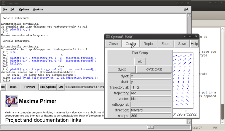
from here you can change the expressions for dx/dt, dy/dt, dy/dx, you can change colours and directions of trajectories (choices of forward, backward, both), change colours for direction arrows and orthogonal curves, starting points for trajectories (the two numbers separated by a space here, not a comma), time increments for t, number of steps used to create an integral curve. You can also look at an integral plots for x(t) and y(t) corresponding to the starting point given (or clicked) by hitting the “plot vs t” button. You can also zoom in or out by hitting the “zoom” button and clicking (or shift+clicking to unzoom), doing something else like hitting the config button will allow you to quit being in zoom mode click for trajectories again. (there might be a better way of doing this btw) You can also save these plots as eps files (you can then tweak these in other vector graphics based programs like Inkscape (free) or Adobe Illustrator etc..)
Interactive sliders
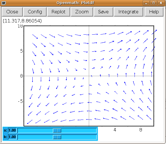
There are many permutations of things you can do (and you will surely find some of these by having a play) but my particular favourite is the option to use sliders allowing you to vary a parameter interactively and seeing what happens to the trajectories without constant replotting. ie:
plotdf([a*y,b*x],[sliders,"a=-1:3,b=-1:3"]);
Hopefully, this has been enough to get people started, and for what it’s worth, the help file (though using xmaxima, you’ll find this in the web-browser version) for this topic has a pretty good gallery of different plots and other parameters I didn’t mention.
just to throw in one last thing in the spirit of experimentation, is the following set of commands:
A:matrix([0,1],[1,0]);
B:matrix([x],[y]);
plotdf([A[1].B,A[2].B);
which is another way of doing the same old
plotdf([y,x]);
where here I’ve made a 2×2 matrix A, a 2×1 matrix B, with A[1], A[2] denoting rows 1 and 2 of A respectively and matrix multiplied the rows of A by B (using A[1].B, A[2].B) to serve as inputs for dx/dt and dy/dt
Tutorial written by Gregory Astley, Mathematics Undergraduate at The University of Manchester.