Walking Randomly

WalkingRandomly is coming up to its 15th Anniversary!  When I started blogging in 2007, I never would have believed that this little corner of the web would still be going in 2022!

As you might have noticed, posting frequency has waned over recent years which is partly to do with Real Life taking over somewhat but also because my professional life has become rather more hectic over the years. When I started posting here, I was a junior research computing specialist and when I left academia in  2019 I was a head of Research Computing for a major UK University!  It was a wild ride.

In 2019 I joined the commercial world with The Numerical Algorithms Group where I spent a lovely couple of years immersing myself in commercial cloud, HPC and numerical computing. 

A new beginning

At the beginning of 2021, in the deepest depths of the pandemic, I was offered the opportunity to join MathWorks, The Makers of MATLAB, to work with academia as a ‘Customer Success Engineer’.  Broadly speaking, I help researchers and educators solve their problems with MATLAB.

Things have been going pretty well and earlier this month they gave me my own blog on MathWorks Central.  Little old me right next to the original developer of MATLAB, Cleve Moler, in the gallery of MathWorks bloggers. 

The new blog is called simply The MATLAB blog but as you might expect from someone who has spent 15 years writing about many aspects of scientific computing, there’s going to be a lot more than just MATLAB on there.  Expect to see posts on subjects such as HPC, Research Software Engineering, C++, Python, GPUs and maybe even a little Fortran!

Here’s a few sample posts from the last few weeks

• How to make a GPU version of this MATLAB program by changing two lines
• Exploring the MATLAB beta for Native Apple Silicon
• Finding if all elements of a matrix are finite, fast!

www.walkingrandomly.com won’t be going away and I’ll still post here from time to time but, for the forseeable future at least, most of my output will be on The MATLAB blog.  

It only took me 15 years but I finally figured out how to get paid for blogging :)

See you around kid. 

The MATLAB community site, MATLAB Central, is celebrating its 20th anniversary with a coding competition where the only aim is to make an interesting image with under 280 characters of code. The 280 character limit ensures that the resulting code is tweetable.  There are a couple of things I really like about the format of this competition, other than the obvious fact that the only aim is to make something pretty!

1. No MATLAB license is required! Sign up for a free MathWorks account and away you go.  You can edit and run code in the browser.
2. Stealing reusing other people’s code is actively encouraged! The competition calls it remixing but GitHub users will recognize it as forking. 

Here’s an example.  I wrote a piece of code to render the Sierpiński triangle – Wikipedia using a simple random algorithm called the Chaos game. 

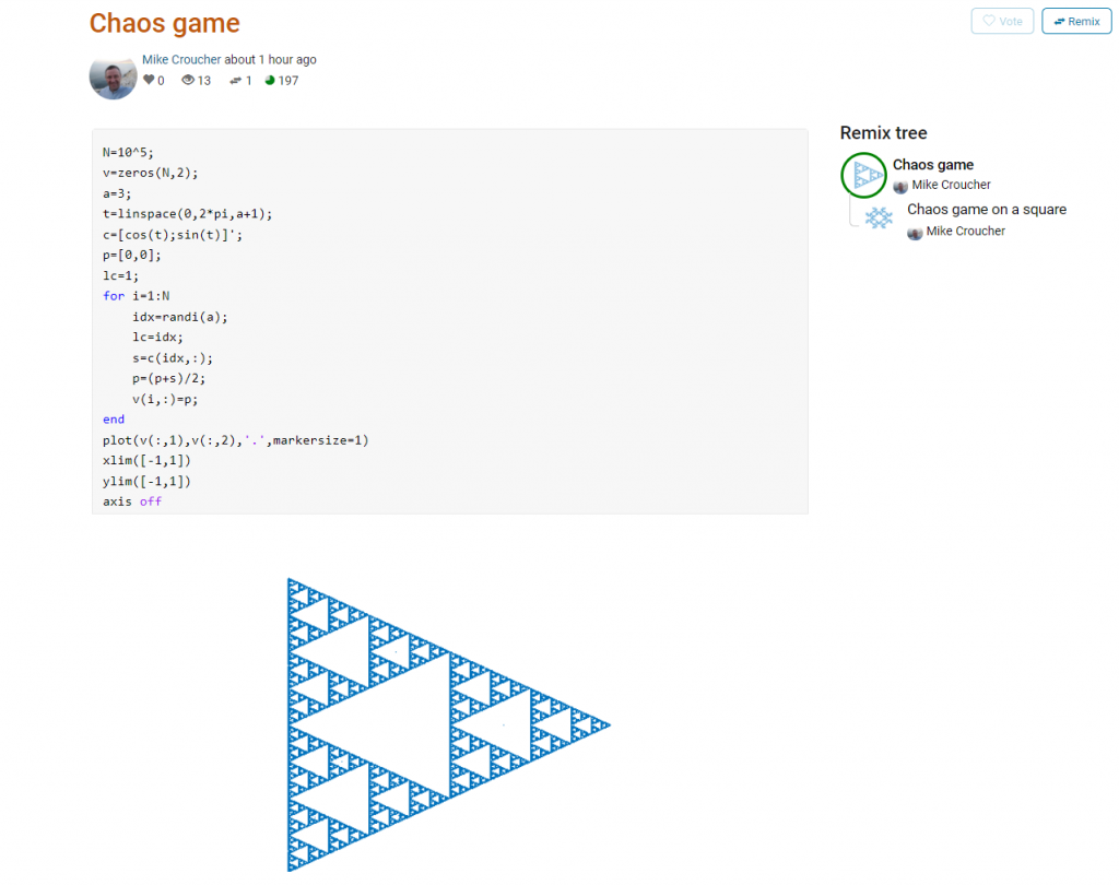
This is about as simple as the Chaos game gets and there are many things that could be done to produce a different image.  As you can see from the Remix tree on the right hand side, I’ve already done one of them by changing a from 3 to 4 and adding some extra code to ensure that the same vertex doesn’t get chosen twice.   This is result:

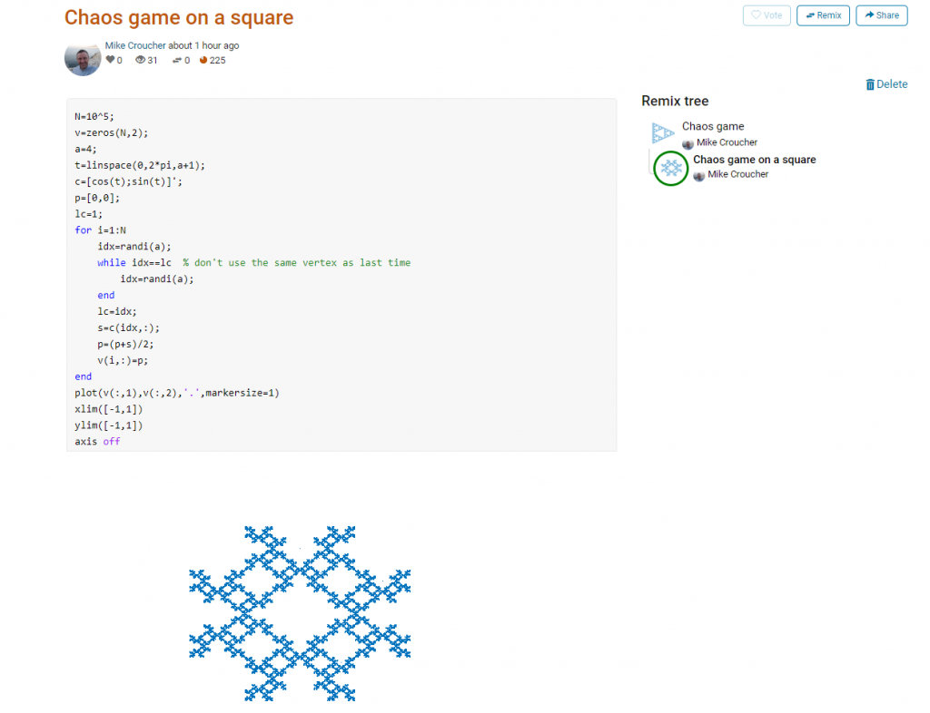
Someone else can now come along, hit the remix button and edit the code to produce something different again.   Some things you might want to try for the chaos game include

• Try changing the value of a which is used in the variables t and c to produce the vertices of a polygon on an enclosing circle.
• Instead of just using the vertices of a polygon, try using the midpoints or another scheme for producing the attractor points completely.
• Try changing the scaling factor — currently p=(p+s)/2;
• Try putting limitations on which vertex is chosen. This remix ensures that the current vertex is different from the last one chosen.
• Each vertex is currently equally likely to be chosen using the code idx=randi(a); Think of ways to change the probabilities.
• Think of ways to colorize the plots.

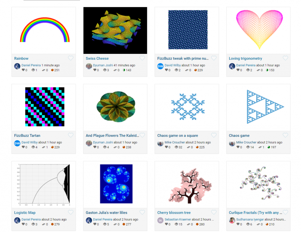
Maybe the chaos game isn’t your thing.  You are free to create your own design from scratch or perhaps you’d prefer to remix some of the other designs in the gallery.

The competition is just a few hours old and there are already some very nice ideas coming out.

Just over 4 years ago I was very happy with the 1.2 Teraflops of single precision performance I measured on my then-new Dell XPS 95600 laptop using MATLAB’s GPU Bench and noted that its performance was on-par with the first supercomputer I supported professionally. Double precision performance stank of course but I had gotten used to that with laptop GPUs!

Fast forward to 2021 and my personal computational landscape has changed substantially. The pandemic has confined me to my home office and high performance laptops don’t have quite the same allure that they did when I was doing most of my interesting computational work in airports and coffee shops. I swapped a 15 inch screen for a 49 inch Ultrawide monitor and my laptop is gathering dust while I enjoy my new Dell desktop with an 8 core Intel i7-11700 and an NVIDIA GTX 3070.

This is the first desktop machine I’ve personally owned for almost two decades and the amount of performance I got for less money than the high spec laptops I used to favour is astonishing! Here are the GPU Bench results using MATLAB 2021a

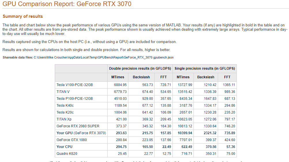
The standout figure is 10,399 Gigaflops for single precision Matrix-Matrix multiplication. At only slightly shy of 10.4 Teraflops that’s almost an order of magnitude faster than the results that impressed me on my laptop 4 years ago!

Double precision performance is nothing to write home about but it never is on consumer NVIDIA GPU cards. I stopped being upset about that years ago!

The other result I find interesting with respect to my personal history of devices is the 622 Gigaflops result for single precision from the Intel i7 CPU. This is getting on for twice as fast as the GPU on my 2015 Apple MacbookPro which managed 349 Gigaflops….a machine I still use today although primarily for Netflix.

My stepchildren are pretty good at mathematics for their age and have recently learned about Pythagora’s theorem

$c=\sqrt{a^2+b^2}$

The fact that they have learned about this so early in their mathematical lives is testament to its importance. Pythagoras is everywhere in computational science and it may well be the case that you’ll need to compute the hypotenuse to a triangle some day.

Fortunately for you, this important computation is implemented in every computational environment I can think of!
It’s almost always called hypot so it will be easy to find.
Here it is in action using Python’s numpy module

import numpy as np
a = 3
b = 4
np.hypot(3,4)

5

When I’m out and about giving talks and tutorials about Research Software Engineering, High Performance Computing and so on, I often get the chance to mention the hypot function and it turns out that fewer people know about this routine than you might expect.

Trivial Calculation? Do it Yourself!

Such a trivial calculation, so easy to code up yourself! Here’s a one-line implementation

def mike_hypot(a,b):
    return(np.sqrt(a*a+b*b))

In use it looks fine

mike_hypot(3,4)

5.0

Overflow and Underflow

I could probably work for quite some time before I found that my implementation was flawed in several places. Here’s one

mike_hypot(1e154,1e154)

inf

You would, of course, expect the result to be large but not infinity. Numpy doesn’t have this problem

np.hypot(1e154,1e154)

1.414213562373095e+154

My function also doesn’t do well when things are small.

a = mike_hypot(1e-200,1e-200)

0.0

but again, the more carefully implemented hypot function in numpy does fine.

np.hypot(1e-200,1e-200)

1.414213562373095e-200

Standards Compliance

Next up — standards compliance. It turns out that there is a an official standard for how hypot implementations should behave in certain edge cases. The IEEE-754 standard for floating point arithmetic has something to say about how any implementation of hypot handles NaNs (Not a Number) and inf (Infinity).

It states that any implementation of hypot should behave as follows (Here’s a human readable summary https://www.agner.org/optimize/nan_propagation.pdf)

hypot(nan,inf) = hypot(inf,nan) = inf

numpy behaves well!

np.hypot(np.nan,np.inf)

inf

np.hypot(np.inf,np.nan)

inf

My implementation does not

mike_hypot(np.inf,np.nan)

nan

So in summary, my implementation is

• Wrong for very large numbers
• Wrong for very small numbers
• Not standards compliant

That’s a lot of mistakes for one line of code! Of course, we can do better with a small number of extra lines of code as John D Cook demonstrates in the blog post What’s so hard about finding a hypotenuse?

Hypot implementations in production

Production versions of the hypot function, however, are much more complex than you might imagine. The source code for the implementation used in openlibm (used by Julia for example) was 132 lines long last time I checked. Here’s a screenshot of part of the implementation I saw for prosterity. At the time of writing the code is at https://github.com/JuliaMath/openlibm/blob/master/src/e_hypot.c

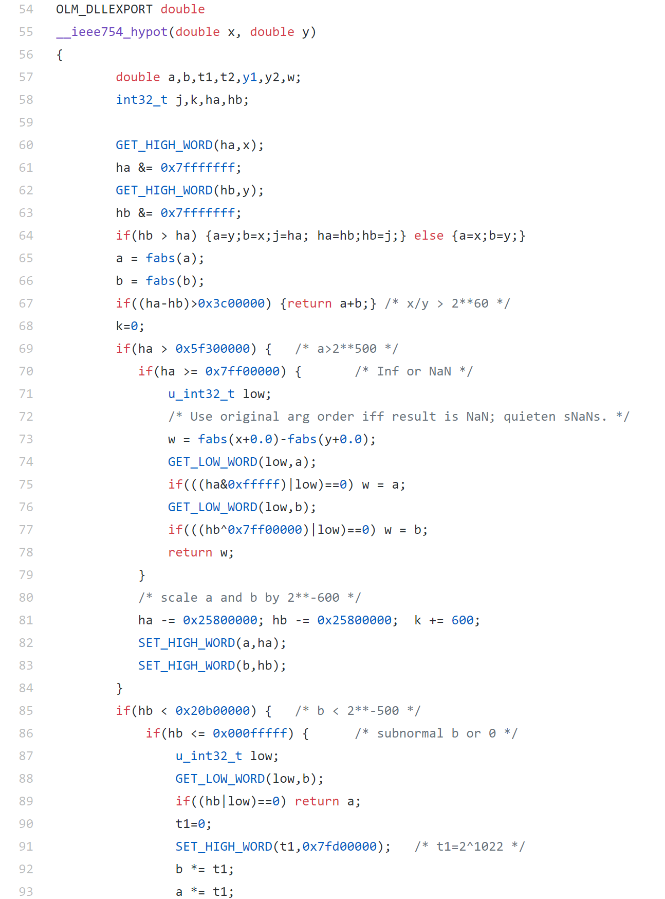
That’s what bullet-proof, bug checked, has been compiled on every platform you can imagine and survived code looks like.

There’s more!

Active Research

When I learned how complex production versions of hypot could be, I shouted out about it on twitter and learned that the story of hypot was far from over!

The implementation of the hypot function is still a matter of active research! See the paper here https://arxiv.org/abs/1904.09481

Is Your Research Software Correct?

Given that such a ‘simple’ computation is so complicated to implement well, consider your own code and ask Is Your Research Software Correct?.

In a recent blog post, Daniel Lemire explicitly demonstrated that vectorising random number generators using SIMD instructions could give useful speed-ups.  This reminded me of the one of the first times I played with the Julia language where I learned that Julia’s random number generator used a SIMD-accelerated implementation of Mersenne Twister called dSFMT to generate random numbers much faster than MATLAB’s Mersenne Twister implementation.

Just recently, I learned that MATLAB now has its own SIMD accelerated version of Mersenne Twister which can be activated like so:

seed=1;
rng(seed,'simdTwister')

This new Mersenne Twister implementation gives different random variates to the original implementation (which I demonstrated is the same as Numpy’s implementation in an older post) as you might expect

>> rng(1,'Twister')
>> rand(1,5)
ans =
0.4170 0.7203 0.0001 0.3023 0.1468
>> rng(1,'simdTwister')
>> rand(1,5)
ans =
0.1194 0.9124 0.5032 0.8713 0.5324

So it’s clearly a different algorithm and, on CPUs that support the relevant instructions, it’s about twice as fast!  Using my very unscientific test code:

format compact
number_of_randoms = 10000000
disp('Timing standard twister')
rng(1,'Twister')
tic;rand(1,number_of_randoms);toc
disp('Timing SIMD twister')
rng(1,'simdTwister')
tic;rand(1,number_of_randoms);toc

gives the following results for a typical run on my Dell XPS 15 9560 which supports AVX instructions

number_of_randoms =
    10000000
Timing standard twister
Elapsed time is 0.101307 seconds.
Timing SIMD twister
Elapsed time is 0.057441 seconds

The MATLAB documentation does not tell us which algorithm their implementation is based on but it seems to be different from Julia’s. In Julia, if we set the seed to 1 as we did for MATLAB and ask for 5 random numbers, we get something different from MATLAB:

julia> using Random
julia> Random.seed!(1);
julia> rand(1,5)
1×5 Array{Float64,2}:
 0.236033  0.346517  0.312707  0.00790928  0.48861

The performance of MATLAB’s new generator is on-par with Julia’s although I’ll repeat that these timing tests are far far from rigorous.

julia> Random.seed!(1);

julia> @time rand(1,10000000);
  0.052981 seconds (6 allocations: 76.294 MiB, 29.40% gc time)

Update
A discussion on twitter determined that this was an issue with Locales. The practical upshot is that we can make R act the same way as the others by doing

Sys.setlocale("LC_COLLATE", "C")

which may or may not be what you should do!

Original post

While working on a project that involves using multiple languages, I noticed some tests failing in one language and not the other. Further investigation revealed that this was essentially because R's default sort order for strings is different from everyone else's.

I have no idea how to say to R 'Use the sort order that everyone else is using'. Suggestions welcomed.

R 3.3.2

sort(c("#b","-b","-a","#a","a","b"))

[1] "-a" "-b" "#a" "#b" "a" "b"

Python 3.6

sorted({"#b","-b","-a","#a","a","b"})

['#a', '#b', '-a', '-b', 'a', 'b']

MATLAB 2018a

sort([{'#b'},{'-b'},{'-a'},{'#a'},{'a'},{'b'}])

ans =
1×6 cell array
{'#a'} {'#b'} {'-a'} {'-b'} {'a'} {'b'}

C++

int main(){ 

std::string mystrs[] = {"#b","-b","-a","#a","a","b"}; 
std::vector<std::string> stringarray(mystrs,mystrs+6);
std::vector<std::string>::iterator it; 

std::sort(stringarray.begin(),stringarray.end());

for(it=stringarray.begin(); it!=stringarray.end();++it) {
   std::cout << *it << " "; 
} 

return 0;
} 

Result:

#a #b -a -b a b

I’m working on some MATLAB code at the moment that I’ve managed to reduce down to a bunch of implicitly parallel functions. This is nice because the data that we’ll eventually throw at it will be represented as a lot of huge matrices.  As such, I’m expecting that if we throw a lot of cores at it, we’ll get a lot of speed-up.  Preliminary testing on local HPC nodes shows that I’m probably right.

During testing and profiling on a smaller data set I thought that it would be fun to run the code on the most powerful single node I can lay my hands on.  In my case that’s an Azure F72s_v2 which I currently get for free thanks to a Microsoft Azure for Research grant I won.

These Azure F72s_v2 machines are NICE! Running Intel Xeon Platinum 8168 CPUs with 72 virtual cores and 144GB of RAM, they put my Macbook Pro to shame! Theoretically, they should be more powerful than any of the nodes I can access on my University HPC system.

So, you can imagine my surprise when the production code ran almost 3 times slower than on my Macbook Pro!

Here’s a Microbenchmark, extracted from the production code, running on MATLAB 2017b on a few machines to show the kind of slowdown I experienced on these super powerful virtual machines.


test_t = rand(8755,1);
test_c = rand(5799,1);
tic;test_res = bsxfun(@times,test_t,test_c');toc
tic;test_res = bsxfun(@times,test_t,test_c');toc


I ran the bsxfun twice and report the fastest since the first call to any function in MATLAB is often slower than subsequent ones for various reasons. This quick and dirty benchmark isn’t exactly rigorous but its good enough to show the issue.

• Azure F72s_v2 (72 vcpus, 144 GB memory) running Windows Server 2016: 0.3 seconds
• Azure F32s_v2 (32 vcpus, 64 GB memory) running Windows Server 2016: 0.29 seconds
• 2014 Macbook Pro running OS X: 0.11 seconds
• Dell XPS 15 9560 laptop running Windows 10: 0.11 seconds
• 8 cores on a node of Sheffield University’s Linux HPC cluster: 0.03 seconds
• 16 cores on a node of Sheffield University’s Linux HPC cluster: 0.015 seconds

After a conversation on twitter, I ran it on Azure twice — once on a 72 vCPU instance and once on a 32 vCPU instance. This was to test if the issue was related to having 2 physical CPUs. The results were pretty much identical.

The results from the University HPC cluster are more in line with what I expected to see — faster than a laptop and good scaling with respect to number of cores.  I tried running it on 32 cores but the benchmark is still in the queue ;)

What’s going on?

I have no idea! I’m stumped to be honest.  Here are some thoughts that occur to me in no particular order

• Maybe it’s an issue with Windows Server 2016. Is there some environment variable I should have set or security option I could have changed? Maybe the Windows version of MATLAB doesn’t get on well with large core counts? I can only test up to 4 on my own hardware and that’s using Windows 10 rather than Windows server.  I need to repeat the experiment using a Linux guest OS.
• Is it an issue related to the fact that there isn’t a 1:1 mapping between physical hardware and virtual cores? Intel Xeon Platinum 8168 CPUs have 24 cores giving 48 hyperthreads so two of them would give me 48 cores and 96 hyperthreads.  They appear to the virtualised OS as 2 x 18 core CPUs with 72 hyperthreads in total.   Does this matter in any way?

My new toy is a 2017 Dell XPS 15 9560 laptop on which I am running Windows 10. Once I got over (and fixed) the annoyance of all the advertising in Windows Home, I quickly starting loving this new device.

To get a handle on its performance, I used GPUBench in MATLAB 2016b and got the following results (This was the best of 4 runs…I note that MTimes performance for the CPU (Host PC), for example, varied between 130 and 150 Glops).

• CPU: Intel Core I7-7700HQ (6M Cache, up to 3.8Ghz)
• GPU: NVIDIA GTX 1050 with 4GB GDDR5

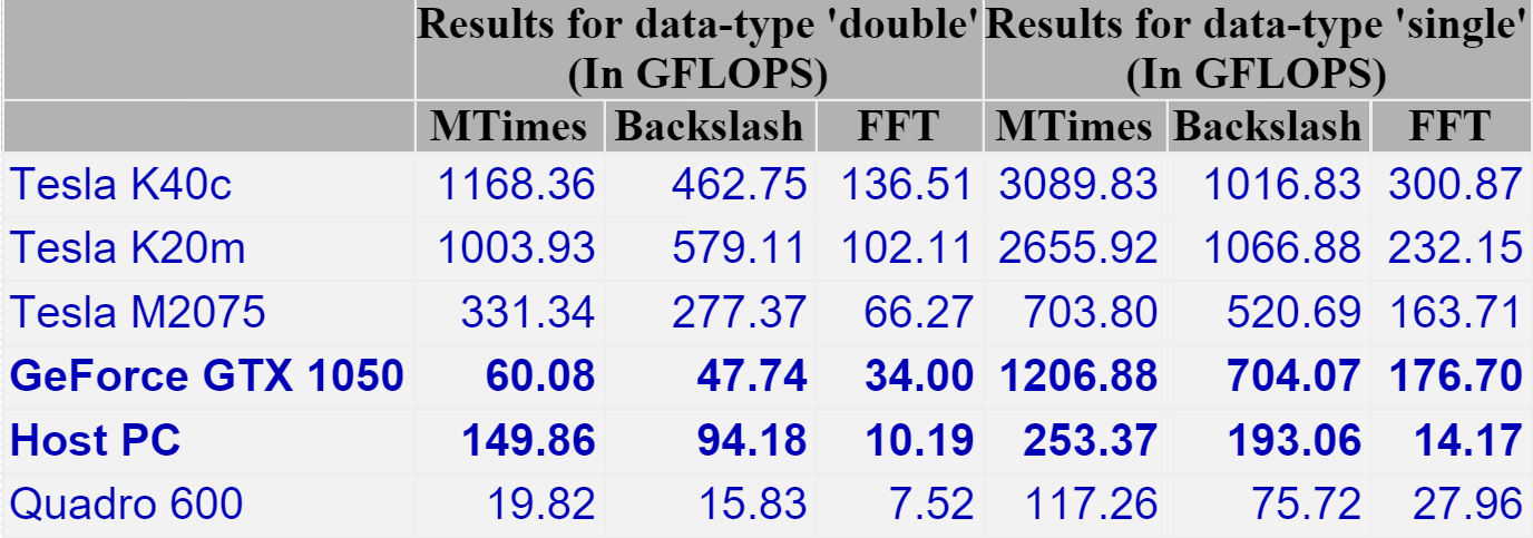
I last did this for my Retina MacBook Pro and am happy to see that the numbers are better across the board. The standout figure for me is the 1206 Gflops (That’s 1.2 Teraflops!) of single precision performance for Matrix-Matrix Multiply.

That figure of 1.2 Teraflops rang a bell for me and it took me a while to realise why…..

My laptop vs Manchester University’s old HPC system – Horace

Old timers like me (I’m almost 40) like to compare modern hardware with bygone supercomputers (1980s Crays vs mobile phones for example) and we know we are truly old when the numbers coming out of laptop benchmarks match the peak theoretical performance of institutional HPC systems we actually used as part of our career.

This has now finally happened to me! I was at the University of Manchester when it commissioned a HPC service called Horace and I was there when it was switched off in 2010 (only 6 and a bit years ago!). It was the University’s primary HPC service with a support team, helpdesk, sysadmins…the lot.  The specs are still available on Manchester’s website:

• 24 nodes, each with 8 cores giving 192 cores in total.
• Each core had a theoretical peak compute performance of 6.4 double precision Gflop/s
• So a node had a theoretical peak performance of 51.2 Gflop/s
• The whole thing could theoretically manage 1.2 Teraflop/s
• It had four special ‘high memory’ nodes with 32Gb RAM each

Good luck getting that 1.2 Teraflops out of it in practice!

I get a big geek-kick out of the fact that my new laptop has the same amount of RAM as one of these ‘big memory’ nodes and that my laptop’s double precision CPU performance is on par with the combined power of 3 of Horace’s nodes. Furthermore, my laptop’s GPU can just about manage 1.2 Teraflop/s of single precision  performance in MATLAB — on par with the total combined power of the HPC system*.

* (I know, I know….Horace’s numbers are for double precision and my GPU numbers are single precision — apples to oranges — but it still astonishes me that the headline numbers are the same — 1.2 Teraflops).

I stumbled across a great list of resources about the R programming language recently – a list called awesome-R. The list said it was inspired by awesome-machine-learning which, in turn, was inspired by awesome-PHP. It turns out that there is a whole network of these lists.

I noticed that there wasn’t a list for MATLAB so started the awesome-MATLAB list. Pull Requests are welcome.

Update: 2nd July 2015 The code in github has moved on a little since this post was written so I changed the link in the text below to the exact commit that produced the results discussed here.

Imagine that you are a very new MATLAB programmer and you have to create an N x N matrix called A where A(i,j) = i+j
Your first attempt at a solution might look like this

N=2000
% Generate a N-by-N matrix where A(i,j) = i + j;
for ii = 1:N
     for jj = 1:N
         A(ii,jj) = ii + jj;
     end
 end

On my current machine (Macbook Pro bought in early 2015), the above loop takes 2.03 seconds. You might think that this is a long time for something so simple and complain that MATLAB is slow. The person you complain to points out that you should preallocate your array before assigning to it.

N=2000
% Generate a N-by-N matrix where A(i,j) = i + j;
A=zeros(N,N);
for ii = 1:N
     for jj = 1:N
         A(ii,jj) = ii + jj;
     end
 end

This now takes 0.049 seconds on my machine – a speed up of over 41 times! MATLAB suddenly doesn’t seem so slow after all.

Word gets around about your problem, however, and seasoned MATLAB-ers see that nested loop, make a funny face twitch and start muttering ‘vectorise, vectorise, vectorise’. Emails soon pile in with vectorised solutions

% Method 1: MESHGRID.
[X, Y] = meshgrid(1:N, 1:N);
A = X + Y;

This takes 0.025 seconds on my machine — a healthy speed-up on the loop-with-preallocation solution. You have to understand the meshgrid command, however, in order to understand what’s going on here. It’s still clear (to me at least) what its doing but not as clear as the nice,obvious double loop. Call me old fashioned but I like loops…I understand them.

% Method 2: Matrix multiplication.
A = (1:N).' * ones(1, N) + ones(N, 1) * (1:N);

This one is MUCH harder to read but you don’t worry about it too much because at 0.032 seconds it’s slower than meshgrid.

% Method 3: REPMAT.
A = repmat(1:N, N, 1) + repmat((1:N).', 1, N);

This one appears to be interesting! At 0.009 seconds, it’s the fastest so far – by a healthy amount!

% Method 4: CUMSUM.
A = cumsum(ones(N)) + cumsum(ones(N), 2);

Coming in at 0.052 seconds, this cumsum solution is slower than the preallocated loop.

% Method 5: BSXFUN.
A = bsxfun(@plus, 1:N, (1:N).');

Ahhh, bsxfun or ‘The Widow-maker function’ as I sometimes refer to it. Responsible for some of the fastest and most unreadable vectorised MATLAB code I’ve ever written. In this case, it brings execution time down to 0.0045 seconds.

Whenever I see something that can be vectorised with a repmat, I try to figure out if I can rewrite it as a bsxfun. The result is usually horrible to look at so I tend to keep the original loop commented out above it as an explanation! This particular example isn’t too bad but bsxfun can quickly get hairy.

Conclusion

Loops in MATLAB aren’t anywhere near as bad as they used to be thanks to advances in JIT compilation but it can often pay, speed-wise, to switch to vectorisation. The price you often pay for this speed-up is that vectorised code can become very difficult to read.

If you’d like the code I ran to get the timings above, it’s on github (link refers to the exact commit used for this post) . Here’s the output from the run I referred to in this post.

Original loop time is 2.025441
Preallocate and loop is 0.048643
Meshgrid time is 0.025277
Matmul time is 0.032069
Repmat time is 0.009030
Cumsum time is 0.051966
bsxfun time is 0.004527

• MATLAB Version: 2015a
• Early 2015 Macbook Pro with 16Gb RAM
• CPU: 2.8Ghz quad core i7 Haswell

This post is based on a demonstration given by Mathwork’s Ken Deeley during a recent session at The University of Sheffield.