
Archive for the ‘Making MATLAB faster’ Category
Just over 4 years ago I was very happy with the 1.2 Teraflops of single precision performance I measured on my then-new Dell XPS 95600 laptop using MATLAB’s GPU Bench and noted that its performance was on-par with the first supercomputer I supported professionally. Double precision performance stank of course but I had gotten used to that with laptop GPUs!
Fast forward to 2021 and my personal computational landscape has changed substantially. The pandemic has confined me to my home office and high performance laptops don’t have quite the same allure that they did when I was doing most of my interesting computational work in airports and coffee shops. I swapped a 15 inch screen for a 49 inch Ultrawide monitor and my laptop is gathering dust while I enjoy my new Dell desktop with an 8 core Intel i7-11700 and an NVIDIA GTX 3070.
This is the first desktop machine I’ve personally owned for almost two decades and the amount of performance I got for less money than the high spec laptops I used to favour is astonishing! Here are the GPU Bench results using MATLAB 2021a
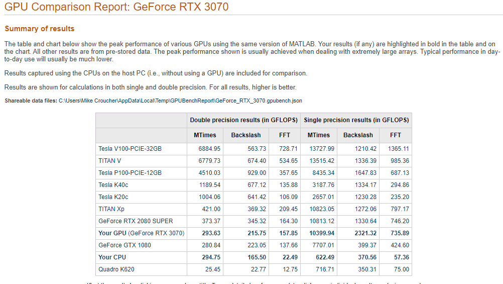
The standout figure is 10,399 Gigaflops for single precision Matrix-Matrix multiplication. At only slightly shy of 10.4 Teraflops that’s almost an order of magnitude faster than the results that impressed me on my laptop 4 years ago!
Double precision performance is nothing to write home about but it never is on consumer NVIDIA GPU cards. I stopped being upset about that years ago!
The other result I find interesting with respect to my personal history of devices is the 622 Gigaflops result for single precision from the Intel i7 CPU. This is getting on for twice as fast as the GPU on my 2015 Apple MacbookPro which managed 349 Gigaflops….a machine I still use today although primarily for Netflix.
In a recent blog post, Daniel Lemire explicitly demonstrated that vectorising random number generators using SIMD instructions could give useful speed-ups. This reminded me of the one of the first times I played with the Julia language where I learned that Julia’s random number generator used a SIMD-accelerated implementation of Mersenne Twister called dSFMT to generate random numbers much faster than MATLAB’s Mersenne Twister implementation.
Just recently, I learned that MATLAB now has its own SIMD accelerated version of Mersenne Twister which can be activated like so:
seed=1;
rng(seed,'simdTwister')
This new Mersenne Twister implementation gives different random variates to the original implementation (which I demonstrated is the same as Numpy’s implementation in an older post) as you might expect
>> rng(1,'Twister')
>> rand(1,5)
ans =
0.4170 0.7203 0.0001 0.3023 0.1468
>> rng(1,'simdTwister')
>> rand(1,5)
ans =
0.1194 0.9124 0.5032 0.8713 0.5324
So it’s clearly a different algorithm and, on CPUs that support the relevant instructions, it’s about twice as fast! Using my very unscientific test code:
format compact
number_of_randoms = 10000000
disp('Timing standard twister')
rng(1,'Twister')
tic;rand(1,number_of_randoms);toc
disp('Timing SIMD twister')
rng(1,'simdTwister')
tic;rand(1,number_of_randoms);toc
gives the following results for a typical run on my Dell XPS 15 9560 which supports AVX instructions
number_of_randoms =
    10000000
Timing standard twister
Elapsed time is 0.101307 seconds.
Timing SIMD twister
Elapsed time is 0.057441 seconds
The MATLAB documentation does not tell us which algorithm their implementation is based on but it seems to be different from Julia’s. In Julia, if we set the seed to 1 as we did for MATLAB and ask for 5 random numbers, we get something different from MATLAB:
julia> using Random
julia> Random.seed!(1);
julia> rand(1,5)
1×5 Array{Float64,2}:
 0.236033  0.346517  0.312707  0.00790928  0.48861
The performance of MATLAB’s new generator is on-par with Julia’s although I’ll repeat that these timing tests are far far from rigorous.
julia> Random.seed!(1);

julia> @time rand(1,10000000);
  0.052981 seconds (6 allocations: 76.294 MiB, 29.40% gc time)
I’m working on some MATLAB code at the moment that I’ve managed to reduce down to a bunch of implicitly parallel functions. This is nice because the data that we’ll eventually throw at it will be represented as a lot of huge matrices. As such, I’m expecting that if we throw a lot of cores at it, we’ll get a lot of speed-up. Preliminary testing on local HPC nodes shows that I’m probably right.
During testing and profiling on a smaller data set I thought that it would be fun to run the code on the most powerful single node I can lay my hands on. In my case that’s an Azure F72s_v2 which I currently get for free thanks to a Microsoft Azure for Research grant I won.
These Azure F72s_v2 machines are NICE! Running Intel Xeon Platinum 8168 CPUs with 72 virtual cores and 144GB of RAM, they put my Macbook Pro to shame! Theoretically, they should be more powerful than any of the nodes I can access on my University HPC system.
So, you can imagine my surprise when the production code ran almost 3 times slower than on my Macbook Pro!
Here’s a Microbenchmark, extracted from the production code, running on MATLAB 2017b on a few machines to show the kind of slowdown I experienced on these super powerful virtual machines.
test_t = rand(8755,1);

test_c = rand(5799,1);

tic;test_res = bsxfun(@times,test_t,test_c');toc

tic;test_res = bsxfun(@times,test_t,test_c');toc
I ran the bsxfun twice and report the fastest since the first call to any function in MATLAB is often slower than subsequent ones for various reasons. This quick and dirty benchmark isn’t exactly rigorous but its good enough to show the issue.
- Azure F72s_v2 (72 vcpus, 144 GB memory) running Windows Server 2016: 0.3 seconds
- Azure F32s_v2 (32 vcpus, 64 GB memory) running Windows Server 2016: 0.29 seconds
- 2014 Macbook Pro running OS X: 0.11 seconds
- Dell XPS 15 9560 laptop running Windows 10: 0.11 seconds
- 8 cores on a node of Sheffield University’s Linux HPC cluster: 0.03 seconds
- 16 cores on a node of Sheffield University’s Linux HPC cluster: 0.015 seconds
After a conversation on twitter, I ran it on Azure twice — once on a 72 vCPU instance and once on a 32 vCPU instance. This was to test if the issue was related to having 2 physical CPUs. The results were pretty much identical.
The results from the University HPC cluster are more in line with what I expected to see — faster than a laptop and good scaling with respect to number of cores. I tried running it on 32 cores but the benchmark is still in the queue ;)
What’s going on?
I have no idea! I’m stumped to be honest. Here are some thoughts that occur to me in no particular order
- Maybe it’s an issue with Windows Server 2016. Is there some environment variable I should have set or security option I could have changed? Maybe the Windows version of MATLAB doesn’t get on well with large core counts? I can only test up to 4 on my own hardware and that’s using Windows 10 rather than Windows server. I need to repeat the experiment using a Linux guest OS.
- Is it an issue related to the fact that there isn’t a 1:1 mapping between physical hardware and virtual cores? Intel Xeon Platinum 8168 CPUs have 24 cores giving 48 hyperthreads so two of them would give me 48 cores and 96 hyperthreads. They appear to the virtualised OS as 2 x 18 core CPUs with 72 hyperthreads in total. Does this matter in any way?
Update: 2nd July 2015 The code in github has moved on a little since this post was written so I changed the link in the text below to the exact commit that produced the results discussed here.
Imagine that you are a very new MATLAB programmer and you have to create an N x N matrix called A where A(i,j) = i+j
Your first attempt at a solution might look like this
N=2000
% Generate a N-by-N matrix where A(i,j) = i + j;
for ii = 1:N
     for jj = 1:N
         A(ii,jj) = ii + jj;
     end
 end
On my current machine (Macbook Pro bought in early 2015), the above loop takes 2.03 seconds. You might think that this is a long time for something so simple and complain that MATLAB is slow. The person you complain to points out that you should preallocate your array before assigning to it.
N=2000
% Generate a N-by-N matrix where A(i,j) = i + j;
A=zeros(N,N);
for ii = 1:N
     for jj = 1:N
         A(ii,jj) = ii + jj;
     end
 end
This now takes 0.049 seconds on my machine – a speed up of over 41 times! MATLAB suddenly doesn’t seem so slow after all.
Word gets around about your problem, however, and seasoned MATLAB-ers see that nested loop, make a funny face twitch and start muttering ‘vectorise, vectorise, vectorise’. Emails soon pile in with vectorised solutions
% Method 1: MESHGRID.
[X, Y] = meshgrid(1:N, 1:N);
A = X + Y;
This takes 0.025 seconds on my machine — a healthy speed-up on the loop-with-preallocation solution. You have to understand the meshgrid command, however, in order to understand what’s going on here. It’s still clear (to me at least) what its doing but not as clear as the nice,obvious double loop. Call me old fashioned but I like loops…I understand them.
% Method 2: Matrix multiplication.
A = (1:N).' * ones(1, N) + ones(N, 1) * (1:N);
This one is MUCH harder to read but you don’t worry about it too much because at 0.032 seconds it’s slower than meshgrid.
% Method 3: REPMAT.
A = repmat(1:N, N, 1) + repmat((1:N).', 1, N);
This one appears to be interesting! At 0.009 seconds, it’s the fastest so far – by a healthy amount!
% Method 4: CUMSUM.
A = cumsum(ones(N)) + cumsum(ones(N), 2);
Coming in at 0.052 seconds, this cumsum solution is slower than the preallocated loop.
% Method 5: BSXFUN.
A = bsxfun(@plus, 1:N, (1:N).');
Ahhh, bsxfun or ‘The Widow-maker function’ as I sometimes refer to it. Responsible for some of the fastest and most unreadable vectorised MATLAB code I’ve ever written. In this case, it brings execution time down to 0.0045 seconds.
Whenever I see something that can be vectorised with a repmat, I try to figure out if I can rewrite it as a bsxfun. The result is usually horrible to look at so I tend to keep the original loop commented out above it as an explanation! This particular example isn’t too bad but bsxfun can quickly get hairy.
Conclusion
Loops in MATLAB aren’t anywhere near as bad as they used to be thanks to advances in JIT compilation but it can often pay, speed-wise, to switch to vectorisation. The price you often pay for this speed-up is that vectorised code can become very difficult to read.
If you’d like the code I ran to get the timings above, it’s on github (link refers to the exact commit used for this post) . Here’s the output from the run I referred to in this post.
Original loop time is 2.025441
Preallocate and loop is 0.048643
Meshgrid time is 0.025277
Matmul time is 0.032069
Repmat time is 0.009030
Cumsum time is 0.051966
bsxfun time is 0.004527
- MATLAB Version: 2015a
- Early 2015 Macbook Pro with 16Gb RAM
- CPU: 2.8Ghz quad core i7 Haswell
This post is based on a demonstration given by Mathwork’s Ken Deeley during a recent session at The University of Sheffield.
Consider the following code
function testpow()
%function to compare integer powers with repeated multiplication

rng default
a=rand(1,10000000)*10;

disp('speed of ^4 using pow')
tic;test4p = a.^4;toc
disp('speed of ^4 using multiply')
tic;test4m = a.*a.*a.*a;toc

disp('maximum difference in results');
max_diff = max(abs(test4p-test4m))

end
On running it on my late 2013 Macbook Air with a Haswell Intel i5 using MATLAB 2013b, I get the following results
speed of ^4 using pow
Elapsed time is 0.527485 seconds.
speed of ^4 using multiply
Elapsed time is 0.025474 seconds.
maximum difference in results
max_diff =
   1.8190e-12
In this case (derived from a real-world case), using repeated multiplication is around twenty times faster than using integer powers in MATLAB. This leads to some questions:-
- Why the huge speed difference?
- Would a similar speed difference be seen in other systems–R, Python, Julia etc?
- Would we see the same speed difference on other operating systems/CPUs?
- Are there any numerical reasons why using repeated multiplication instead of integer powers is a bad idea?
While working on someone’s MATLAB code today there came a point when it was necessary to generate a vector of powers. For example, [a a^2 a^3….a^10000] where a=0.999
a=0.9999;
y=a.^(1:10000);
This isn’t the only way one could form such a vector and I was curious whether or not an alternative method might be faster. On my current machine we have:
>> tic;y=a.^(1:10000);toc
Elapsed time is 0.001526 seconds.
>> tic;y=a.^(1:10000);toc
Elapsed time is 0.001529 seconds.
>> tic;y=a.^(1:10000);toc
Elapsed time is 0.001716 seconds.
Let’s look at the last result in the vector y
>> y(end)
ans =
   0.367861046432970
So, 0.0015-ish seconds to beat.
>> tic;y1=cumprod(ones(1,10000)*a);toc
Elapsed time is 0.000075 seconds.
>> tic;y1=cumprod(ones(1,10000)*a);toc
Elapsed time is 0.000075 seconds.
>> tic;y1=cumprod(ones(1,10000)*a);toc
Elapsed time is 0.000075 seconds.
soundly beaten! More than a factor of 20 in fact. Let’s check out that last result
>> y1(end)
ans =
   0.367861046432969
Only a difference in the 15th decimal place–I’m happy with that. What I’m wondering now, however, is will my faster method ever cause me grief?
This is only an academic exercise since this is not exactly a hot spot in the code!
I was recently working on some MATLAB code with Manchester University’s David McCormick. Buried deep within this code was a function that was called many,many times…taking up a significant amount of overall run time. We managed to speed up an important part of this function by almost a factor of two (on his machine) simply by inserting two brackets….a new personal record in overall application performance improvement per number of keystrokes.
The code in question is hugely complex, but the trick we used is really very simple. Consider the following MATLAB code
>> a=rand(4000);
>> c=12.3;
>> tic;res1=c*a*a';toc
Elapsed time is 1.472930 seconds.
With the insertion of just two brackets, this runs quite a bit faster on my Ivy Bridge quad-core desktop.
>> tic;res2=c*(a*a');toc
Elapsed time is 0.907086 seconds.
So, what’s going on? Well, we think that in the first version of the code, MATLAB first calculates c*a to form a temporary matrix (let’s call it temp here) and then goes on to find temp*a’. However, in the second version, we think that MATLAB calculates a*a’ first and in doing so it takes advantage of the fact that the result of multiplying a matrix by its transpose will be symmetric which is where we get the speedup.
Another demonstration of this phenomena can be seen as follows
>> a=rand(4000);
>> b=rand(4000);
>> tic;a*a';toc
Elapsed time is 0.887524 seconds.
>> tic;a*b;toc
Elapsed time is 1.473208 seconds.
>> tic;b*b';toc
Elapsed time is 0.966085 seconds.
Note that the symmetric matrix-matrix multiplications are faster than the general, non-symmetric one.
Ever since I took a look at GPU accelerating simple Monte Carlo Simulations using MATLAB, I’ve been disappointed with the performance of its GPU random number generator. In MATLAB 2012a, for example, it’s not much faster than the CPU implementation on my GPU hardware. Consider the following code
function gpuRandTest2012a(n)

mydev=gpuDevice();
disp('CPU - Mersenne Twister');
tic
CPU = rand(n);
toc

sg = parallel.gpu.RandStream('mrg32k3a','Seed',1);
parallel.gpu.RandStream.setGlobalStream(sg);
disp('GPU - mrg32k3a');
tic
Rg = parallel.gpu.GPUArray.rand(n);
wait(mydev);
toc
Running this on MATLAB 2012a on my laptop gives me the following typical times (If you try this out yourself, the first run will always be slower for various reasons I’ll not go into here)
>> gpuRandTest2012a(10000)
CPU - Mersenne Twister
Elapsed time is 1.330505 seconds.
GPU - mrg32k3a
Elapsed time is 1.006842 seconds.
Running the same code on MATLAB 2012b, however, gives a very pleasant surprise with typical run times looking like this
CPU - Mersenne Twister
Elapsed time is 1.590764 seconds.
GPU - mrg32k3a
Elapsed time is 0.185686 seconds.
So, generation of random numbers using the GPU is now over 7 times faster than CPU generation on my laptop hardware–a significant improvment on the previous implementation.
New generators in 2012b
The MATLAB developers went a little further in 2012b though. Not only have they significantly improved performance of the mrg32k3a combined multiple recursive generator, they have also implemented two new GPU random number generators based on the Random123 library. Here are the timings for the generation of 100 million random numbers in MATLAB 2012b
- Get the code – gpuRandTest2012b.m
CPU - Mersenne Twister
Elapsed time is 1.370252 seconds.
GPU - mrg32k3a
Elapsed time is 0.186152 seconds.
GPU - Threefry4x64-20
Elapsed time is 0.145144 seconds.
GPU - Philox4x32-10
Elapsed time is 0.129030 seconds.
Bear in mind that I am running this on the relatively weak GPU of my laptop! If anyone runs it on something stronger, I’d love to hear of your results.
- Laptop model: Dell XPS L702X
- CPU: Intel Core i7-2630QM @2Ghz software overclockable to 2.9Ghz. 4 physical cores but total 8 virtual cores due to Hyperthreading.
- GPU: GeForce GT 555M with 144 CUDA Cores. Graphics clock: 590Mhz. Processor Clock:1180 Mhz. 3072 Mb DDR3 Memeory
- RAM: 8 Gb
- OS: Windows 7 Home Premium 64 bit.
- MATLAB: 2012a/2012b
I recently got access to a shiny new (new to me at least) set of compilers, The Portland PGI compiler suite which comes with a great set of technologies to play with including AVX vector support, CUDA for x86 and GPU pragma-based acceleration. So naturally, it wasn’t long before I wondered if I could use the PGI suite as compilers for MATLAB mex files. The bad news is that The Mathworks don’t support the PGI Compilers out of the box but that leads to the good news…I get to dig down and figure out how to add support for unsupported compilers.
In what follows I made use of MATLAB 2012a on 64bit Windows 7 with Version 12.5 of the PGI Portland Compiler Suite.
In order to set up a C mex-compiler in MATLAB you execute the following
mex -setup
which causes MATLAB to execute a Perl script at C:\Program Files\MATLAB\R2012a\bin\mexsetup.pm. This script scans the directory C:\Program Files\MATLAB\R2012a\bin\win64\mexopts looking for Perl scripts with the extension .stp and running whatever it finds. Each .stp file looks for a particular compiler. After all .stp files have been executed, a list of compilers found gets returned to the user. When the user chooses a compiler, the corresponding .bat file gets copied to the directory returned by MATLAB’s prefdir function. This sets up the compiler for use. All of this is nicely documented in the mexsetup.pm file itself.
So, I’ve had my first crack at this and the results are the following two files.
These are crude, and there’s probably lots missing/wrong but they seem to work. Copy them to C:\Program Files\MATLAB\R2012a\bin\win64\mexopts. The location of the compiler is hard-coded in pgi.stp so you’ll need to change the following line if your compiler location differs from mine
my $default_location = "C:\\Program Files\\PGI\\win64\\12.5\\bin";
Now, when you do mex -setup, you should get an entry PGI Workstation 12.5 64bit 12.5 in C:\Program Files\PGI\win64\12.5\bin which you can select as normal.
An example compilation and some details.
Let’s compile the following very simple mex file, mex_sin.c, using the PGI compiler which does little more than take an elementwise sine of the input matrix.
#include <math.h>
#include "mex.h"

void mexFunction( int nlhs, mxArray *plhs[], int nrhs, const mxArray *prhs[] )
{
    double *in,*out;
    double dist,a,b;
    int rows,cols,outsize;
    int i,j,k;

    /*Get pointers to input matrix*/
    in = mxGetPr(prhs[0]);
    /*Get rows and columns of input*/
    rows = mxGetM(prhs[0]);
    cols = mxGetN(prhs[0]);

    /* Create output matrix */
    outsize = rows*cols;
    plhs[0] = mxCreateDoubleMatrix(rows, cols, mxREAL);
    /* Assign pointer to the output */
    out = mxGetPr(plhs[0]);

    for(i=0;i<outsize;i++){
        out[i] = sin(in[i]);
    }

}
Compile using the -v switch to get verbose information about the compilation
mex sin_mex.c -v
You’ll see that the compiled mex file is actually a renamed .dll file that was compiled and linked with the following flags
pgcc -c -Bdynamic  -Minfo -fast
pgcc --Mmakedll=export_all  -L"C:\Program Files\MATLAB\R2012a\extern\lib\win64\microsoft" libmx.lib libmex.lib libmat.lib
The switch –Mmakedll=export_all is actually not supported by PGI which makes this whole setup doubly unsupported! However, I couldn’t find a way to export the required symbols without modifying the mex source code so I lived with it. Maybe I’ll figure out a better way in the future. Let’s try the new function out
>> a=[1 2 3];
>> mex_sin(a)
Invalid MEX-file 'C:\Work\mex_sin.mexw64': The specified module could not be found.
The reason for the error message is that a required PGI .dll file, pgc.dll, is not on my system path so I need to do the following in MATLAB.
setenv('PATH', [getenv('PATH') ';C:\Program Files\PGI\win64\12.5\bin\']);
This fixes things
>> mex_sin(a)
ans =
    0.8415    0.9093    0.1411
Performance
I took a quick look at the performance of this mex function using my quad-core, Sandy Bridge laptop. I highly doubted that I was going to beat MATLAB’s built in sin function (which is highly optimised and multithreaded) with so little work and I was right:
>> a=rand(1,100000000);
>> tic;mex_sin(a);toc
Elapsed time is 1.320855 seconds.
>> tic;sin(a);toc
Elapsed time is 0.486369 seconds.
That’s not really a fair comparison though since I am purposely leaving mutithreading out of the PGI mex equation for now. It’s a much fairer comparison to compare the exact same mex file using different compilers so let’s do that. I created three different compiled mex routines from the source code above using the three compilers installed on my laptop and performed a very crude time test as follows
>> a=rand(1,100000000);
>> tic;mex_sin_pgi(a);toc              %PGI 12.5 run 1
Elapsed time is 1.317122 seconds.
>> tic;mex_sin_pgi(a);toc              %PGI 12.5 run 2
Elapsed time is 1.338271 seconds.

>> tic;mex_sin_vs(a);toc               %Visual Studio 2008 run 1
Elapsed time is 1.459463 seconds.
>> tic;mex_sin_vs(a);toc
Elapsed time is 1.446947 seconds.      %Visual Studio 2008 run 2

>> tic;mex_sin_intel(a);toc             %Intel Compiler 12.0 run 1
Elapsed time is 0.907018 seconds.
>> tic;mex_sin_intel(a);toc             %Intel Compiler 12.0 run 2
Elapsed time is 0.860218 seconds.
PGI did a little better than Visual Studio 2008 but was beaten by Intel. I’m hoping that I’ll be able to get more performance out of the PGI compiler as I learn more about the compilation flags.
Getting PGI to make use of SSE extensions
Part of the output of the mex sin_mex.c -v compilation command is the following notice
mexFunction:
     23, Loop not vectorized: data dependency
This notice is a result of the -Minfo compilation switch and indicates that the PGI compiler can’t determine if the in and out arrays overlap or not. If they don’t overlap then it would be safe to unroll the loop and make use of SSE or AVX instructions to make better use of my Sandy Bridge processor. This should hopefully speed things up a little.
As the programmer, I am sure that the two arrays don’t overlap so I need to give the compiler a hand. One way to do this would be to modify the pgi.dat file to include the compilation switch -Msafeptr which tells the compiler that arrays never overlap anywhere. This might not be a good idea since it may not always be true so I decided to be more cautious and make use of the restrict keyword. That is, I changed the mex source code so that
double *in,*out;
becomes
double * restrict in,* restrict out;
Now when I compile using the PGI compiler, the notice from -Mifno becomes
mexFunction:
     23, Generated 3 alternate versions of the loop
         Generated vector sse code for the loop
         Generated a prefetch instruction for the loop
which demonstrates that the compiler is much happier! So, what did this do for performance?
>> tic;mex_sin_pgi(a);toc
Elapsed time is 1.450002 seconds.
>> tic;mex_sin_pgi(a);toc
Elapsed time is 1.460536 seconds.
This is slower than when SSE instructions weren’t being used which isn’t what I was expecting at all! If anyone has any insight into what’s going on here, I’d love to hear from you.
Future Work
I’m happy that I’ve got this compiler working in MATLAB but there is a lot to do including:
- Tidy up the pgi.dat and pgi.stp files so that they look and act more professionally.
- Figure out the best set of compiler switches to use– it is almost certain that what I’m using now is sub-optimal since I am new to the PGI compiler.
- Get OpenMP support working. I tried using the -Mconcur compilation flag which auto-parallelised the loop but it crashed MATLAB when I ran it. This needs investigating
- Get PGI accelerator support working so I can offload work to the GPU.
- Figure out why the SSE version of this function is slower than the non-SSE version
- Figure out how to determine whether or not the compiler is emitting AVX instructions. The documentation suggests that if the compiler is called on a Sandy Bridge machine, and if vectorisation is possible then it will produce AVX instructions but AVX is not mentioned in the output of -Minfo. Nothing changes if you explicity set the target to Sandy Bridge with the compiler switch –tp sandybridge–64.
Look out for more articles on this in the future.
Related WalkingRandomly Articles
- Which MATLAB functions make use of multithreading?
- Using Intel’s SPMD Compiler (ispc) with MATLAB on Linux
- Parallel MATLAB with OpenMP mex files
- MATLAB mex functions using the NAG C Library
My setup
- Laptop model: Dell XPS L702X
- CPU: Intel Core i7-2630QM @2Ghz software overclockable to 2.9Ghz. 4 physical cores but total 8 virtual cores due to Hyperthreading.
- GPU: GeForce GT 555M with 144 CUDA Cores. Graphics clock: 590Mhz. Processor Clock:1180 Mhz. 3072 Mb DDR3 Memeory
- RAM: 8 Gb
- OS: Windows 7 Home Premium 64 bit.
- MATLAB: 2012a
- PGI Compiler: 12.5
This article is the third part of a series where I look at rewriting a particular piece of MATLAB code using various techniques. The introduction to the series is here and the introduction to the larger series of GPU articles for MATLAB is here.
Last time I used The Mathwork’s Parallel Computing Toolbox in order to modify a simple correlated asset calculation to run on my laptop’s GPU rather than its CPU. Performance was not as good as I had hoped and I never managed to get my laptop’s GPU (an NVIDIA GT555M) to beat the CPU using functions from the parallel computing toolbox. Transferring the code to a much more powerful Tesla GPU card resulted in a four times speed-up compared to the CPU in my laptop.
This time I’ll take a look at AccelerEyes’ Jacket, a third party GPU solution for MATLAB.
Attempt 1 – Make as few modifications as possible
I started off just as I did for the parallel computing toolbox GPU port; by taking the best CPU-only code from part 1 (optimised_corr2.m) and changing a load of data-types from double to gdouble in order to get the calculation to run on my laptop’s GPU using Jacket v1.8.1 and MATLAB 2010b. I also switched to using the GPU versions of various functions such as grandn instead of randn for example. Functions such as cumprod needed no modifications at all since they are nicely overloaded; if the argument to cumprod is of type double then the calculation happens on the CPU whereas if it is gdouble then it happens on the GPU.
Now, one thing that I don’t like about Jacket’s implementation is that many of the functions return single precision numbers by default. For example, if you do
a=grand(1,10)
then you end up with 10 numbers of type gsingle. To get double precision numbers you have to do
grandn(1,10,'double')
Now you may be thinking ‘what’s the big deal? – it’s just a bit of syntax so get over it’ and I guess that would be a fair comment. Supporting single precision also allows users of legacy GPUs to get in on the GPU-accelerated action which is a good thing. The problem as I see it is that almost everything else in MATLAB uses double precision numbers as the default and so it’s easy to get caught out. I would much rather see functions such as grand return double precision by default with the option to use single precision if required–just like almost every other MATLAB function out there.
The result of my ‘port’ is GPU_jacket_corr1.m
One thing to note in this version, along with all subsequent Jacket versions, is the following command that appears at the very end of the program.
gsync;
This is very important if you want to get meaningful timing results since it ensures that all GPU computations have finished before execution continues. See the Jacket documentation on gysnc and this blog post on timing Jacket code for more details.
The other thing I’ll mention is that, in this version, I do this:
Corr = [1 0.4; 0.4 1];
UpperTriangle=gdouble(chol(Corr));
instead of
Corr = gdouble([1 0.4; 0.4 1]);
UpperTriangle=chol(Corr);
In other words, I do the cholesky decomposition on the CPU and move the results to the GPU rather than doing the calculation on the GPU. This is mainly because I don’t have access to a Jacket DLA license but it’s probably the best thing to do anyway since such a small decomposition probably won’t happen any faster on the GPU.
So, how does it perform. I ran it three times with the now usual parameters of 100000 simulations done in blocks of 125 (see the CPU version for how I came to choose 125)
>> tic;GPU_jacket_corr1;toc
Elapsed time is 40.691888 seconds.
>> tic;GPU_jacket_corr1;toc
Elapsed time is 32.096796 seconds.
>> tic;GPU_jacket_corr1;toc
Elapsed time is 32.039982 seconds.
Just like the Parallel Computing Toolbox, the first run is slower because of GPU warmup overheads. Also, just like the PCT, performance stinks! It’s clearly not enough, in this case at least, to blindly throw in a few gdoubles and hope for the best. It is worth noting, however, that this case is nowhere near as bad as the 900+ seconds we saw in the similar parallel computing toolbox version.
Jacket has punished me for being stupid (or optimistic if you want to be polite to me) but not as much as the PCT did.
Attempt 2 – Convert from a script to a function
When working with the Parallel Computing Toolbox I demonstrated that a switch from a script to a function yielded some speed-up. This wasn’t the case with the Jacket version of the code. The functional version, GPU_jacket_corr2.m, showed no discernable speed improvement compared to the script.
%Warm up run performed previously
>> tic;GPU_jacket_corr2(100000,125);toc
Elapsed time is 32.230638 seconds.
>> tic;GPU_jacket_corr2(100000,125);toc
Elapsed time is 32.179734 seconds.
>> tic;GPU_jacket_corr2(100000,125);toc
Elapsed time is 32.114864 seconds.
Attempt 3 – One big matrix multiply!
The original version of this calculation performs thousands of very small matrix multiplications and last time we saw that switching to a single, large matrix multiplication brought significant speed improvements on the GPU. Modifying the code to do this with Jacket is a very similar process to doing it for the PCT so I’ll omit the details and just present the code, GPU_jacket_corr3.m
%Warm up runs performed previously
>> tic;GPU_jacket_corr3(100000,125);toc
Elapsed time is 2.041111 seconds.
>> tic;GPU_jacket_corr3(100000,125);toc
Elapsed time is 2.025450 seconds.
>> tic;GPU_jacket_corr3(100000,125);toc
Elapsed time is 2.032390 seconds.
Now that’s more like it! Finally we have a GPU version that runs faster than the CPU on my laptop. We can do better, however, since the block size of 125 was chosen especially for my CPU. With this Jacket version bigger is better and we get much more speed-up by switching to a block size of 25000 (I run out of memory on the GPU if I try even bigger block sizes).
%Warm up runs performed previously
>> tic;GPU_jacket_corr3(100000,25000);toc
Elapsed time is 0.749945 seconds.
>> tic;GPU_jacket_corr3(100000,25000);toc
Elapsed time is 0.749333 seconds.
>> tic;GPU_jacket_corr3(100000,25000);toc
Elapsed time is 0.749556 seconds.
Now this is exciting! My laptop GPU with Jacket 1.8.1 is faster than a high-end Tesla card using the parallel computing toolbox for this calculation. My excitement was short lived, however, when I looked at the resulting distribution. The random number generator in Jacket 1.8.1 gave a completely different distribution when compared to generators from other sources (I tried two CPU generators from The Mathworks and one from The Numerical Algorithms Group). The only difference in the code that generated the results below is the random number generator used.
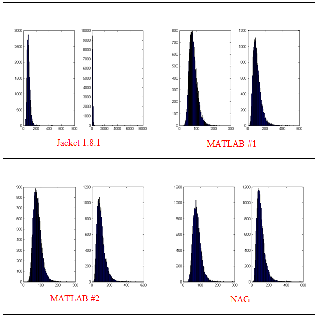
- The results shown in these plots were for only 20,000 simulations rather than the 100,000 I’ve been using elsewhere in this post. I found this bug in the development stage of these posts where I was using a smaller number of simulations.
- Jacket 1.8.1 is using Jackets old grandn function with the ‘double’ option set
- MATLAB #1 is using MATLAB’s randn using the Comb Recursive algorithm on the CPU
- MATLAB #2 is using MATLAB’s randn using the default Mersenne Twister on the CPU
- NAG is using a Wichman-Hill generator
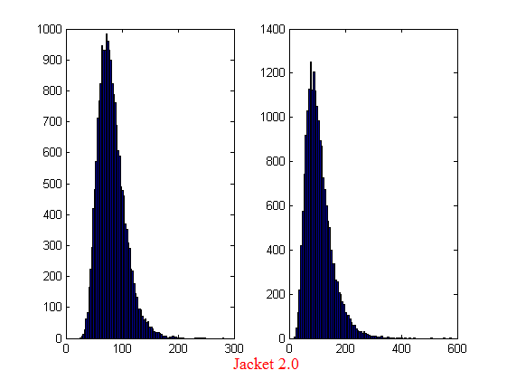
I sent my code to AccelerEye’s customer support who confirmed that this seemed to be a bug in their random number generator (an in-house Mersenne Twister implementation). Less than a week later they offered me a new preview of Jacket from their Nightly builds where the old RNG had been replaced with the Mersenne Twister implementation produced by NVidia and I’m happy to confirm that not only does this fix the results for my code but it goes even faster! Superb customer service!
This new RNG is now the default in version 2.0 of Jacket. Here’s the distribution I get for 20,000 simulations (to stay in line with the plots shown above).
Switching back to 100,000 simulations to stay in line with all of the other benchmarks in this series gives the following times on my laptop’s GPU
%Warm up runs performed previously
>> tic;prices=GPU_jacket_corr3(100000,25000);toc
Elapsed time is 0.696891 seconds.
>> tic;prices=GPU_jacket_corr3(100000,25000);toc
Elapsed time is 0.697596 seconds.
>> tic;prices=GPU_jacket_corr3(100000,25000);toc
Elapsed time is 0.697312 seconds.
This is almost 5 times faster than the 3.42 seconds managed by the best CPU version from part 1. I sent my code to AccelerEyes and asked them to run it on a more powerful GPU, a Tesla C2075, and these are the results they sent back
Elapsed time is 5.246249 seconds. %warm up run
Elapsed time is 0.158165 seconds.
Elapsed time is 0.156529 seconds.
Elapsed time is 0.156522 seconds.
Elapsed time is 0.156501 seconds.
So, the Tesla is 4.45 times faster than my laptop’s GPU for this application and a very useful 21.85 times faster than my laptop’s CPU.
Results Summary
- Best CPU Result on laptop (i7-2630GM)with pure MATLAB code – 3.42 seconds
- Best GPU Result with PCT on laptop (GT555M) – 4.04 seconds
- Best GPU Result with PCT on Tesla M2070 – 0.85 seconds
- Best GPU Result with Jacket on laptop (GT555M) – 0.7 seconds
- Best GPU Result with Jacket on Tesla M2075 – 0.16 seconds
Test System Specification
- Laptop model: Dell XPS L702X
- CPU:Intel Core i7-2630QM @2Ghz software overclockable to 2.9Ghz. 4 physical cores but total 8 virtual cores due to Hyperthreading.
- GPU:GeForce GT 555M with 144 CUDA Cores. Graphics clock: 590Mhz. Processor Clock:1180 Mhz. 3072 Mb DDR3 Memeory
- RAM: 8 Gb
- OS: Windows 7 Home Premium 64 bit.
- MATLAB: 2011b
Acknowledgements
Thanks to Yong Woong Lee of the Manchester Business School as well as various employees at AccelerEyes for useful discussions and advice. Any mistakes that remain are all my own.