
Archive for the ‘tutorials’ Category
My stepchildren are pretty good at mathematics for their age and have recently learned about Pythagora’s theorem
$c=\sqrt{a^2+b^2}$
The fact that they have learned about this so early in their mathematical lives is testament to its importance. Pythagoras is everywhere in computational science and it may well be the case that you’ll need to compute the hypotenuse to a triangle some day.
Fortunately for you, this important computation is implemented in every computational environment I can think of!
It’s almost always called hypot so it will be easy to find.
Here it is in action using Python’s numpy module
import numpy as np
a = 3
b = 4
np.hypot(3,4)

5
When I’m out and about giving talks and tutorials about Research Software Engineering, High Performance Computing and so on, I often get the chance to mention the hypot function and it turns out that fewer people know about this routine than you might expect.
Trivial Calculation? Do it Yourself!
Such a trivial calculation, so easy to code up yourself! Here’s a one-line implementation
def mike_hypot(a,b):
    return(np.sqrt(a*a+b*b))
In use it looks fine
mike_hypot(3,4)

5.0
Overflow and Underflow
I could probably work for quite some time before I found that my implementation was flawed in several places. Here’s one
mike_hypot(1e154,1e154)

inf
You would, of course, expect the result to be large but not infinity. Numpy doesn’t have this problem
np.hypot(1e154,1e154)

1.414213562373095e+154
My function also doesn’t do well when things are small.
a = mike_hypot(1e-200,1e-200)

0.0
but again, the more carefully implemented hypot function in numpy does fine.
np.hypot(1e-200,1e-200)

1.414213562373095e-200
Standards Compliance
Next up — standards compliance. It turns out that there is a an official standard for how hypot implementations should behave in certain edge cases. The IEEE-754 standard for floating point arithmetic has something to say about how any implementation of hypot handles NaNs (Not a Number) and inf (Infinity).
It states that any implementation of hypot should behave as follows (Here’s a human readable summary https://www.agner.org/optimize/nan_propagation.pdf)
hypot(nan,inf) = hypot(inf,nan) = inf
numpy behaves well!
np.hypot(np.nan,np.inf)

inf

np.hypot(np.inf,np.nan)

inf
My implementation does not
mike_hypot(np.inf,np.nan)

nan
So in summary, my implementation is
- Wrong for very large numbers
- Wrong for very small numbers
- Not standards compliant
That’s a lot of mistakes for one line of code! Of course, we can do better with a small number of extra lines of code as John D Cook demonstrates in the blog post What’s so hard about finding a hypotenuse?
Hypot implementations in production
Production versions of the hypot function, however, are much more complex than you might imagine. The source code for the implementation used in openlibm (used by Julia for example) was 132 lines long last time I checked. Here’s a screenshot of part of the implementation I saw for prosterity. At the time of writing the code is at https://github.com/JuliaMath/openlibm/blob/master/src/e_hypot.c
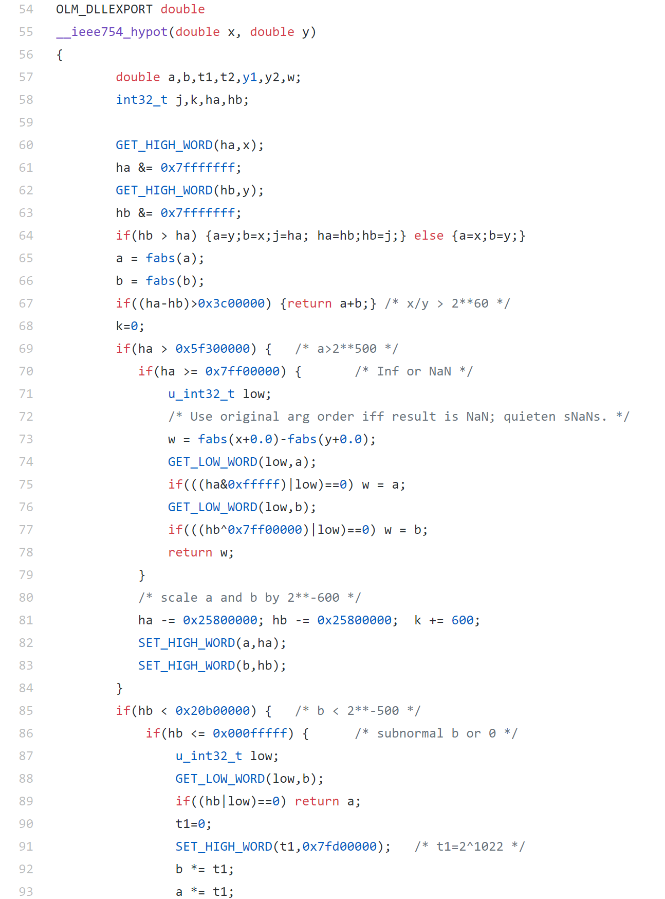
That’s what bullet-proof, bug checked, has been compiled on every platform you can imagine and survived code looks like.
There’s more!
Active Research
When I learned how complex production versions of hypot could be, I shouted out about it on twitter and learned that the story of hypot was far from over!
The implementation of the hypot function is still a matter of active research! See the paper here https://arxiv.org/abs/1904.09481

Is Your Research Software Correct?
Given that such a ‘simple’ computation is so complicated to implement well, consider your own code and ask Is Your Research Software Correct?.
What is Second Order Cone Programming (SOCP)?
Second Order Cone Programming (SOCP) problems are a type of optimisation problem that have applications in many areas of science, finance and engineering. A summary of the type of problems that can make use of SOCP, including things as diverse as designing antenna arrays, finite impulse response (FIR) filters and structural equilibrium problems can be found in the paper ‘Applications of Second Order Cone Programming’ by Lobo et al. There are also a couple of examples of using SOCP for portfolio optimisation in the GitHub repository of the Numerical Algorithms Group (NAG).
A large scale SOCP solver was one of the highlights of the Mark 27 release of the NAG library (See here for a poster about its performance). Those who have used the NAG library for years will expect this solver to have interfaces in Fortran and C and, of course, they are there. In addition to this is the fact that Mark 27 of the NAG Library for Python was released at the same time as the Fortran and C interfaces which reflects the importance of Python in today’s numerical computing landscape.
Here’s a quick demo of how the new SOCP solver works in Python. The code is based on a notebook in NAG’s PythonExamples GitHub repository.
NAG’s handle_solve_socp_ipm function (also known as e04pt) is a solver from the NAG optimization modelling suite for large-scale second-order cone programming (SOCP) problems based on an interior point method (IPM).
$$
\begin{array}{ll}
{\underset{x \in \mathbb{R}^{n}}{minimize}\ } & {c^{T}x} \\
\text{subject to} & {l_{A} \leq Ax \leq u_{A}\text{,}} \\
& {l_{x} \leq x \leq u_{x}\text{,}} \\
& {x \in \mathcal{K}\text{,}} \\
\end{array}
$$
where $\mathcal{K} = \mathcal{K}^{n_{1}} \times \cdots \times \mathcal{K}^{n_{r}} \times \mathbb{R}^{n_{l}}$ is a Cartesian product of quadratic (second-order type) cones and $n_{l}$-dimensional real space, and $n = \sum_{i = 1}^{r}n_{i} + n_{l}$ is the number of decision variables. Here $c$, $x$, $l_x$ and $u_x$ are $n$-dimensional vectors.
$A$ is an $m$ by $n$ sparse matrix, and $l_A$ and $u_A$ and are $m$-dimensional vectors. Note that $x \in \mathcal{K}$ partitions subsets of variables into quadratic cones and each $\mathcal{K}^{n_{i}}$ can be either a quadratic cone or a rotated quadratic cone. These are defined as follows:
- Quadratic cone:
$$
\mathcal{K}_{q}^{n_{i}} := \left\{ {z = \left\{ {z_{1},z_{2},\ldots,z_{n_{i}}} \right\} \in {\mathbb{R}}^{n_{i}} \quad\quad : \quad\quad z_{1}^{2} \geq \sum\limits_{j = 2}^{n_{i}}z_{j}^{2},\quad\quad\quad z_{1} \geq 0} \right\}\text{.}
$$
- Rotated quadratic cone:
$$
\mathcal{K}_{r}^{n_{i}} := \left\{ {z = \left\{ {z_{1},z_{2},\ldots,z_{n_{i}}} \right\} \in {\mathbb{R}}^{n_{i}}\quad\quad:\quad \quad\quad 2z_{1}z_{2} \geq \sum\limits_{j = 3}^{n_{i}}z_{j}^{2}, \quad\quad z_{1} \geq 0, \quad\quad z_{2} \geq 0} \right\}\text{.}
$$
For a full explanation of this routine, refer to e04ptc in the NAG Library Manual
Using the NAG SOCP Solver from Python
This example, derived from the documentation for the handle_set_group function solves the following SOCP problem
minimize $${10.0x_{1} + 20.0x_{2} + x_{3}}$$
from naginterfaces.base import utils
from naginterfaces.library import opt

# The problem size:
n = 3

# Create the problem handle:
handle = opt.handle_init(nvar=n)

# Set objective function
opt.handle_set_linobj(handle, cvec=[10.0, 20.0, 1.0])
subject to the bounds
$$
\begin{array}{rllll}
{- 2.0} & \leq & x_{1} & \leq & 2.0 \\
{- 2.0} & \leq & x_{2} & \leq & 2.0 \\
\end{array}
$$
# Set box constraints
opt.handle_set_simplebounds(
    handle,
    bl=[-2.0, -2.0, -1.e20],
    bu=[2.0, 2.0, 1.e20]
)
the general linear constraints
& & {- 0.1x_{1}} & – & {0.1x_{2}} & + & x_{3} & \leq & 1.5 & & \\
1.0 & \leq & {- 0.06x_{1}} & + & x_{2} & + & x_{3} & & & & \\
\end{array}
# Set linear constraints
opt.handle_set_linconstr(
    handle,
    bl=[-1.e20, 1.0],
    bu=[1.5, 1.e20],
    irowb=[1, 1, 1, 2, 2, 2],
    icolb=[1, 2, 3, 1, 2, 3],
    b=[-0.1, -0.1, 1.0, -0.06, 1.0, 1.0]
    );
and the cone constraint
$$\left( {x_{3},x_{1},x_{2}} \right) \in \mathcal{K}_{q}^{3}\text{.}$$
# Set cone constraint
opt.handle_set_group(
    handle,
    gtype='Q',
    group=[ 3,1, 2],
    idgroup=0
);
We set some algorithmic options. For more details on the options available, refer to the routine documentation
# Set some algorithmic options.
for option in [
        'Print Options = NO',
        'Print Level = 1'
]:
    opt.handle_opt_set(handle, option)

# Use an explicit I/O manager for abbreviated iteration output:
iom = utils.FileObjManager(locus_in_output=False)
Finally, we call the solver
# Call SOCP interior point solver
result = opt.handle_solve_socp_ipm(handle, io_manager=iom)
 ------------------------------------------------
  E04PT, Interior point method for SOCP problems
 ------------------------------------------------

 Status: converged, an optimal solution found
 Final primal objective value -1.951817E+01
 Final dual objective value   -1.951817E+01
The optimal solution is
result.x
array([-1.26819151, -0.4084294 , 1.3323379 ])
and the objective function value is
result.rinfo[0]
-19.51816515094211
Finally, we clean up after ourselves by destroying the handle
# Destroy the handle:
opt.handle_free(handle)
As you can see, the way to use the NAG Library for Python interface follows the mathematics quite closely.
NAG also recently added support for the popular cvxpy modelling language that I’ll discuss another time.
Links
I’m working on optimising some R code written by a researcher at University of Sheffield and its very much a war of attrition! There’s no easily optimisable hotspot and there’s no obvious way to leverage parallelism. Progress is being made by steadily identifying places here and there where we can do a little better. 10% here and 20% there can eventually add up to something worth shouting about.
One such micro-optimisation we discovered involved multiplying two matrices together where one of them needed to be transposed. Here’s a minimal example.
#Set random seed for reproducibility
set.seed(3)

# Generate two random n by n matrices
n = 10
a = matrix(runif(n*n,0,1),n,n)
b = matrix(runif(n*n,0,1),n,n)

# Multiply the matrix a by the transpose of b
c = a %*% t(b)
When the speed of linear algebra computations are an issue in R, it makes sense to use a version that is linked to a fast implementation of BLAS and LAPACK and we are already doing that on our HPC system.
Here, I am using version 3.3.3 of Microsoft R Open which links to Intel’s MKL (an implementation of BLAS and LAPACK) on a Windows laptop.
In R, there is another way to do the computation c = a %*% t(b) — we can make use of the tcrossprod function (There is also a crossprod function for when you want to do t(a) %*% b)
c_new = tcrossprod(a,b)
Let’s check for equality
c_new == c
[,1] [,2] [,3] [,4] [,5] [,6] [,7] [,8] [,9] [,10]
[1,] TRUE TRUE TRUE TRUE TRUE TRUE TRUE TRUE TRUE TRUE
[2,] TRUE TRUE TRUE TRUE TRUE TRUE TRUE TRUE TRUE TRUE
[3,] TRUE TRUE TRUE TRUE TRUE TRUE TRUE TRUE TRUE TRUE
[4,] TRUE TRUE TRUE TRUE TRUE TRUE TRUE TRUE TRUE TRUE
[5,] TRUE TRUE TRUE TRUE TRUE TRUE TRUE TRUE TRUE TRUE
[6,] TRUE TRUE TRUE TRUE TRUE TRUE TRUE TRUE TRUE TRUE
[7,] TRUE TRUE TRUE TRUE TRUE TRUE TRUE TRUE TRUE TRUE
[8,] TRUE TRUE TRUE TRUE TRUE TRUE TRUE TRUE TRUE TRUE
[9,] TRUE TRUE TRUE TRUE TRUE TRUE TRUE TRUE TRUE TRUE
[10,] TRUE TRUE TRUE TRUE TRUE TRUE TRUE TRUE TRUE TRUE
Sometimes, when comparing the two methods you may find that some of those entries are FALSE which may worry you!
If that happens, computing the difference between the two results should convince you that all is OK and that the differences are just because of numerical noise. This happens sometimes when dealing with floating point arithmetic (For example, see https://www.walkingrandomly.com/?p=5380).
Let’s time the two methods using the microbenchmark package.
install.packages('microbenchmark')
library(microbenchmark)
We time just the matrix multiplication part of the code above:
microbenchmark(
original = a %*% t(b),
tcrossprod = tcrossprod(a,b)
)


Unit: nanoseconds
expr min lq mean median uq max neval
original 2918 3283 3491.312 3283 3647 18599 1000
tcrossprod 365 730 756.278 730 730 10576 1000
We are only saving microseconds here but that’s more than a factor of 4 speed-up in this small matrix case. If that computation is being performed a lot in a tight loop (and for our real application, it was), it can add up to quite a difference.
As the matrices get bigger, the speed-benefit in percentage terms gets lower but tcrossprod always seems to be the faster method. For example, here are the results for 1000 x 1000 matrices
#Set random seed for reproducibility
set.seed(3)

# Generate two random n by n matrices
n = 1000
a = matrix(runif(n*n,0,1),n,n)
b = matrix(runif(n*n,0,1),n,n)

microbenchmark(
original = a %*% t(b),
tcrossprod = tcrossprod(a,b)
)

Unit: milliseconds
expr min lq mean median uq max neval
original 18.93015 26.65027 31.55521 29.17599 31.90593 71.95318 100
tcrossprod 13.27372 18.76386 24.12531 21.68015 23.71739 61.65373 100
The cost of not using an optimised version of BLAS and LAPACK
While writing this blog post, I accidentally used the CRAN version of R. The recently released version 3.4. Unlike Microsoft R Open, this is not linked to the Intel MKL and so matrix multiplication is rather slower.
For our original 10 x 10 matrix example we have:
library(microbenchmark)
#Set random seed for reproducibility
set.seed(3)

# Generate two random n by n matrices
n = 10
a = matrix(runif(n*n,0,1),n,n)
b = matrix(runif(n*n,0,1),n,n)

microbenchmark(
original = a %*% t(b),
tcrossprod = tcrossprod(a,b)
)

Unit: microseconds
       expr   min    lq    mean median     uq    max neval
   original 3.647 3.648 4.22727  4.012 4.1945 22.611   100
 tcrossprod 1.094 1.459 1.52494  1.459 1.4600  3.282   100
Everything is a little slower as you might expect and the conclusion of this article — tcrossprod(a,b) is faster than a %*% t(b) — seems to still be valid.
However, when we move to 1000 x 1000 matrices, this changes
library(microbenchmark)
#Set random seed for reproducibility
set.seed(3)

# Generate two random n by n matrices
n = 1000
a = matrix(runif(n*n,0,1),n,n)
b = matrix(runif(n*n,0,1),n,n)

microbenchmark(
original = a %*% t(b),
tcrossprod = tcrossprod(a,b)
)

Unit: milliseconds
       expr      min       lq     mean   median       uq       max neval
   original 546.6008 587.1680 634.7154 602.6745 658.2387  957.5995   100
 tcrossprod 560.4784 614.9787 658.3069 634.7664 685.8005 1013.2289   100
As expected, both results are much slower than when using the Intel MKL-lined version of R (~600 milliseconds vs ~31 milliseconds) — nothing new there. More disappointingly, however, is that now tcrossprod is slightly slower than explicitly taking the transpose.
As such, this particular micro-optimisation might not be as effective as we might like for all versions of R.
One of the great things about being a Research Software Engineer is the diversity of work you can get involved with. I specialise in smaller interventions which means that I can be working with physicists on Monday, engineers on Tuesday, geneticists on Wednesday….you get the idea.
Last month, I got to work with some Ecologists along with Anna Krystalli. We undertook the arduous journey from Sheffield down to Exeter to deliver talks and workshops at a post-conference symposium on reproducibility in science, organised by Malika Ihle and Isabel Winney, at the International Symposium on Behavioural Ecology.
I gave my talk, Is your research software correct?, and also delivered a workshop on using projects and version control using R and RStudio in the Code Cafe style. For the full write up of the day, see the excellent blog post by Anna over at the Mozilla Science Lab blog.
Updates : More resources
- Elevating the status of code in Ecology. Thanks to @katerererena for pointing this one out to me.
- Anna Krystalli’s course material
Like many people, I was excited to learn about the new Linux subsystem in Windows announced by Microsoft earlier this year (See Bash on Windows: The scripting game just changed).
Along with others, I’ve been playing with it on the Windows Insider builds but now that the Windows Anniversary Update has been released, everyone can get in on the action.
Activating the Linux Subsystem in Windows
Once you’ve updated to the Anniversary Update of Windows, here’s what you need to do.
Open settings

In settings, click on Update and Security

In Update and Security, click on For developers in the left hand pane. Then click on Developer mode.

Take note of the Use developer features warning and click Yes if you are happy. Developer mode gives you greater power, and with great power comes great responsibility.

Reboot the machine (may not be necessary here but it’s what I did).
Search for Features and click on Turn Windows features on or off

Tick Windows Subsystem for Linux (Beta) and click OK

When it’s finished churning, reboot the machine.
Launch cmd.exe

Type bash, press enter and follow the instructions
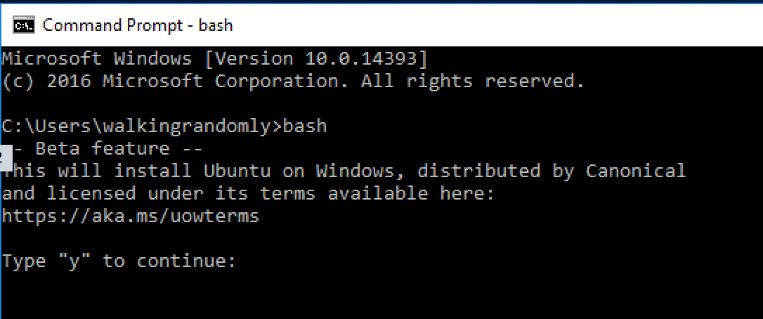
The linux subsystem will be downloaded from the windows store and you’ll be asked to create a Unix username and password.
Try something linux-y
The short version of what’s available is ‘Every userland tool that’s available for Ubuntu’ with the caveat that anything requiring a GUI won’t work.
This isn’t emulation, it isn’t cygwin, it’s something else entirely. It’s very cool!
The gcc compiler isn’t installed by default so let’s fix that:
sudo apt-get install gcc
Using your favourite terminal based editor (I used vi), enter the following ‘Hello World’ code in C and call it hello.c.
/* Hello World program */

#include

int main()
{
    printf("Hello World from C\n");

    return(0);
}
Compile using gcc
gcc hello.c -o hello
Run the executable
./hello
Hello World from C
Now, transfer the executable to a modern Ubuntu machine (I just emailed it to myself) and run it there.
That’s right – you just wrote and compiled a C-program on a Windows machine and ran it on a Linux machine.
Now install cowsay — because you can:
sudo apt-get install cowsay
cowsay 'Hello from Windows'
 ____________________
< Hello from Windows >
 --------------------
        \   ^__^
         \  (oo)\_______
            (__)\       )\/\
                ||----w |
                ||     ||
Update 1:
I was challenged by @linuxlizard to do a follow up tutorial that showed how to install the scientific Python stack — Numpy, SciPy etc.
@walkingrandomly Follow up with HOWTO on installing NumPy, SiPy, Pillow, etc. :-)
— David Poole (@linuxlizard) August 5, 2016
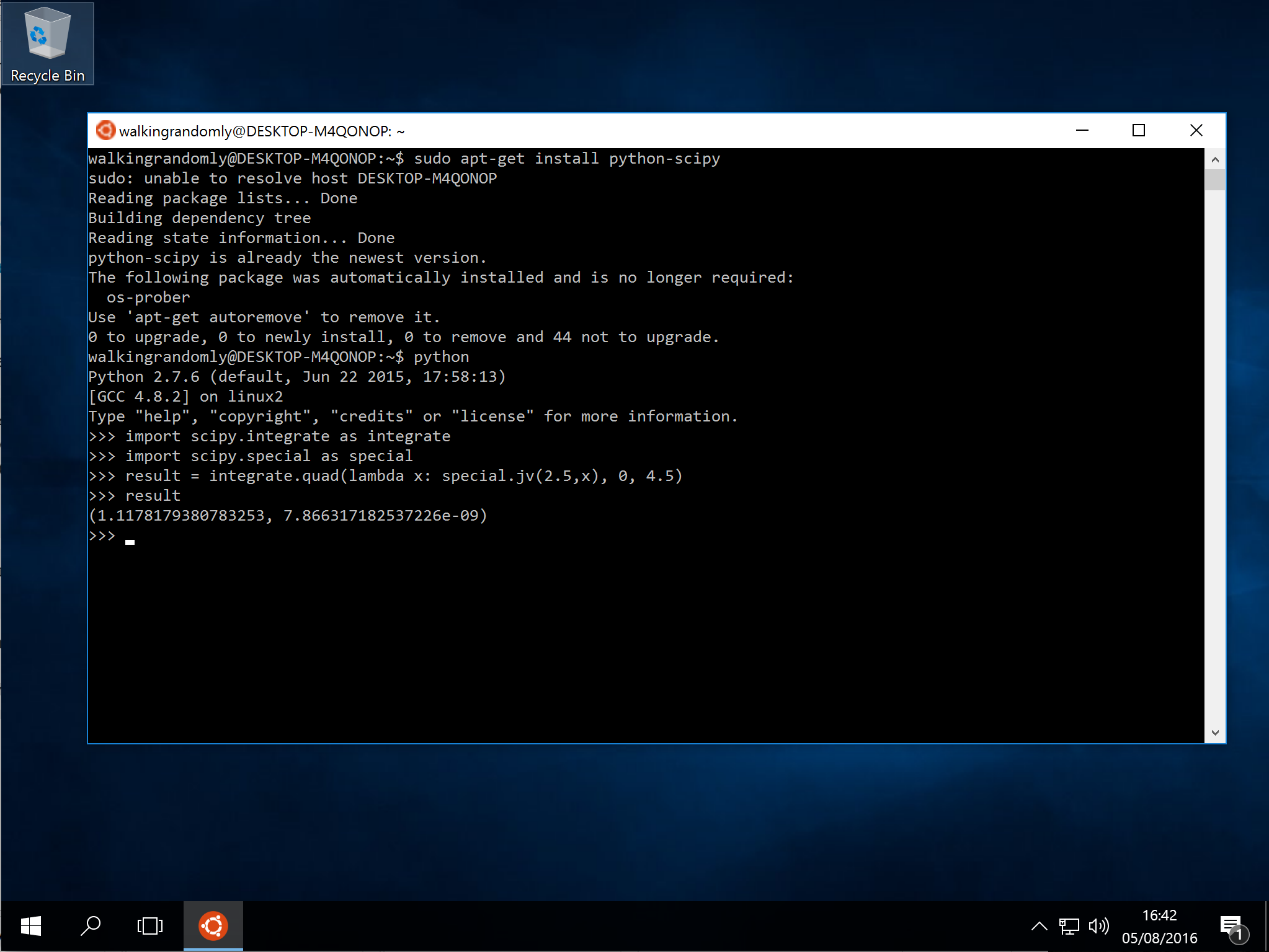
It’s all there :)
sudo apt-get install python-scipy
Update 2
TensorFlow on LinuxOnWindows is also easy: http://www.hanselman.com/blog/PlayingWithTensorFlowOnWindows.aspx
It is possible to write quick, interactive demonstrations in a variety of languages these days. Functions such as Mathematica’s Manipulate, Sage Math’s interact and IPython’s interact allow programmers to write functional graphical user interfaces with just a few lines of code.
Earlier this week, I hosted a session in the Faculty of Engineering at The University of Sheffield where Maplesoft showed us, among other things, their version of this technology. This blog post is an extension of my notes from this part of the session.
- The Maple Worksheet for this blog post is available on github.
The series command expands a function as a power series around a point. For example, let’s expand sin(x) as a power series around the point x=0.
series(sin(x), x = 0, 10)

If we try to plot this, we get an error message
plot(series(sin(x), x = 0, 10), x = -2*Pi .. 2*Pi, y = -3 .. 3)

Warning, unable to evaluate the function to numeric values in the region; see the plotting command's help page to ensure the calling sequence is correct
This is because the output of the series command is a series data structure — something that the plot function cannot handle. We can, however, convert this to a polynomial which is something that the plot function can handle
convert(series(sin(x), x = 0, 10), polynom)

Wrapping the above with plot gives:
plot(convert(series(sin(x), x = 0, 10), polynom), x = -2*Pi .. 2*Pi, y = -3 .. 3);

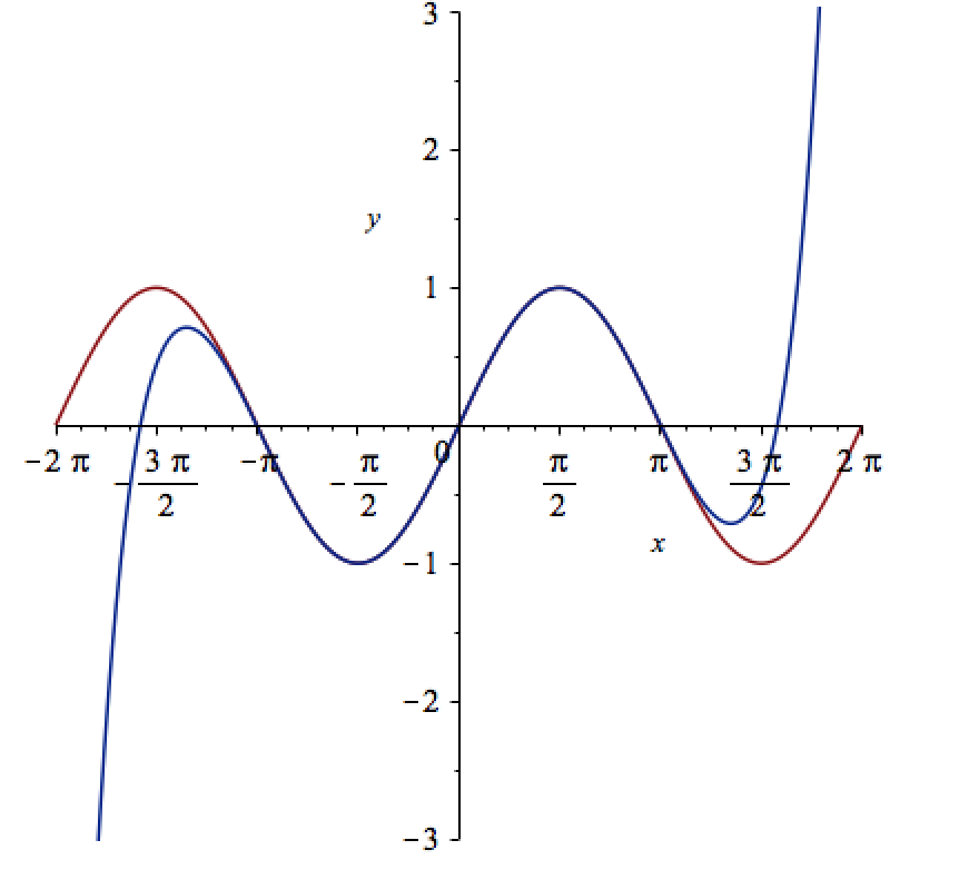
Let’s see how close this is to the sin(x) curve by plotting them both together
plot([sin(x), convert(series(sin(x), x = 0, 10), polynom)], x = -2*Pi .. 2*Pi, y = -3 .. 3);
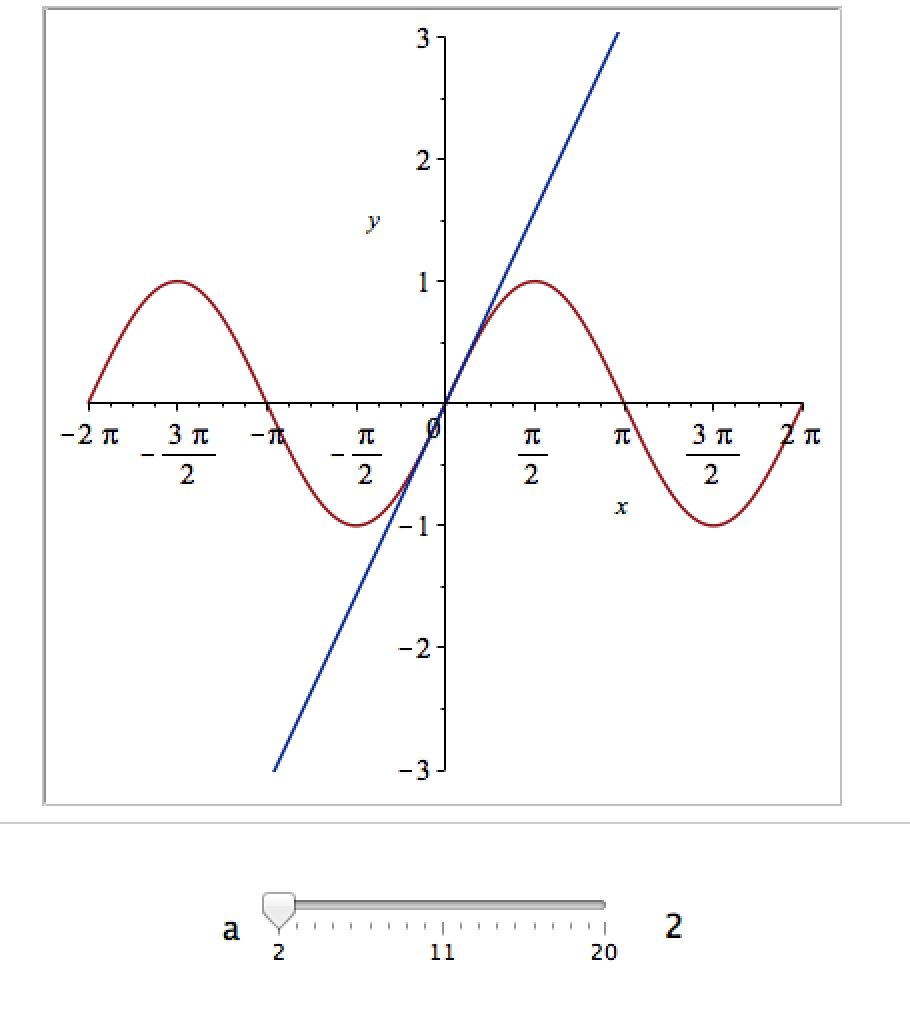
It would be nice if we could see how the approximation varies as we vary the number of terms in the expansion. Change the value 10 to a parameter a, pass the whole thing to the Explore function and we get an interactive widget.
Explore(plot([sin(x), convert(series(sin(x), x = 0, a), polynom)], x = -2*Pi .. 2*Pi, y = -3 .. 3), parameters = [a = 2 .. 20]);
Here’s a screenshot of it:
Adding extra parameters
It would also be nice to vary the point we expand around. Change the value 0 to b and add an extra parameter to Explore to get two sliders instead of one:
Explore(plot([sin(x), convert(series(sin(x), x = b, a), polynom)], x = -2*Pi .. 2*Pi, y = -3 .. 3), parameters = [a = 2 .. 20, b = -2*Pi .. 2*Pi]);
To see what this looks like, open the companion worksheet in Maple.
Adding labels to the sliders
We can change the labels on the sliders as follows
Explore(plot([sin(x), convert(series(sin(x), x = b, a), polynom)], x = -2*Pi .. 2*Pi, y = -3 .. 3), parameters = [[a = 2 .. 20, label = `Number Of Terms`], [b = -2*Pi .. 2*Pi, label = `Expansion location`]]);
To see what this looks like, open the companion worksheet in Maple.
Adding initial values
Finally, let’s set some starting values for each slider
Explore(plot([sin(x), convert(series(sin(x), x = b, a), polynom)], x = -2*Pi .. 2*Pi, y = -3 .. 3), parameters = [[a = 2 .. 20, label = `Number Of Terms`], [b = -2*Pi .. 2*Pi, label = `Expansion location`]], initialvalues = [a = 2, b = 1]);
The resulting interactive widget looks like this:

Not bad for one line of code!
Upload to the Maple Cloud
At The University of Sheffield, we are lucky because all of our staff and students have access to Maple on both university-owned and personally-owned equipment. If your audience isn’t as fortunate, they can access the resulting worksheet on the Maple Cloud.
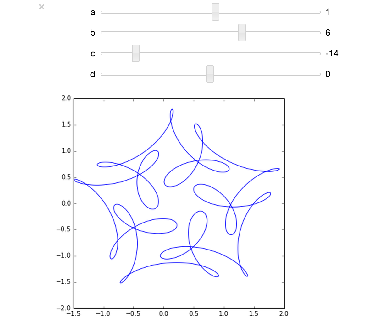
The ever-superb John D. Cook recently found this lovely looking curve in a book he’s currently reading
John posted some Python code that reproduced this curve. I stole borrowed his code, put it in a Jupyter notebook and wrapped it in an interactive widget to allow me to play with the parameters and see what other curves I could come up with. The result looks like this.
If you’d like something where those sliders work, you need to run the notebook I’ve created in Project Jupyter. Here are 2 ways to do that.
- Download the notebook from github
- Method 1: Upload this notebook to Try Jupyter.
- Method 2: Install Anaconda Python on your machine. Launch the notebook and open the file downloaded above.
Once you have the notebook open, click on Cell->Run All and play with the sliders that pop up.
Other posts about these curves:
- Random cyclic curves – Includes code written in Haskell
- A geogebra applet
I occasionally get emails from researchers saying something like this
‘My MATLAB code takes a week to run and the cleaner/cat/my husband keeps switching off my machine before it’s completed — could you help me make the code go faster please so that I can get my results in between these events’
While I am more than happy to try to optimise the code in question, what these users really need is some sort of checkpointing scheme. Checkpointing is also important for users of high performance computing systems that limit the length of each individual job.
The solution – Checkpointing (or ‘Assume that your job will frequently be killed’)
The basic idea behind checkpointing is to periodically save your program’s state so that, if it is interrupted, it can start again where it left off rather than from the beginning. In order to demonstrate some of the principals involved, I’m going to need some code that’s sufficiently simple that it doesn’t cloud what I want to discuss. Let’s add up some numbers using a for-loop.
%addup.m
%This is not the recommended way to sum integers in MATLAB -- we only use it here to keep things simple
%This version does NOT use checkpointing

mysum=0;
for count=1:100
    mysum = mysum + count;
    pause(1);           %Let's pretend that this is a complicated calculation
    fprintf('Completed iteration %d \n',count);
end

fprintf('The sum is %f \n',mysum);
Using a for-loop to perform an addition like this is something that I’d never usually suggest in MATLAB but I’m using it here because it is so simple that it won’t get in the way of understanding the checkpointing code.
If you run this program in MATLAB, it will take about 100 seconds thanks to that pause statement which is acting as a proxy for some real work. Try interrupting it by pressing CTRL-C and then restart it. As you might expect, it will always start from the beginning:
>> addup
Completed iteration 1
Completed iteration 2
Completed iteration 3
Operation terminated by user during addup (line 6)

>> addup
Completed iteration 1
Completed iteration 2
Completed iteration 3
Operation terminated by user during addup (line 6)
This is no big deal when your calculation only takes 100 seconds but is going to be a major problem when the calculation represented by that pause statement becomes something like an hour rather than a second.
Let’s now look at a version of the above that makes use of checkpointing.
%addup_checkpoint.m
if exist( 'checkpoint.mat','file' ) % If a checkpoint file exists, load it
    fprintf('Checkpoint file found - Loading\n');
    load('checkpoint.mat')

else %otherwise, start from the beginning
    fprintf('No checkpoint file found - starting from beginning\n');
    mysum=0;
    countmin=1;
end

for count = countmin:100
    mysum = mysum + count;
    pause(1);           %Let's pretend that this is a complicated calculation

    %save checkpoint
    countmin = count+1;  %If we load this checkpoint, we want to start on the next iteration
    fprintf('Saving checkpoint\n');
    save('checkpoint.mat');

    fprintf('Completed iteration %d \n',count);
end
fprintf('The sum is %f \n',mysum);
Before you run the above code, the checkpoint file checkpoint.mat does not exist and so the calculation starts from the beginning. After every iteration, a checkpoint file is created which contains every variable in the MATLAB workspace. If the program is restarted, it will find the checkpoint file and continue where it left off. Our code now deals with interruptions a lot more gracefully.
>> addup_checkpoint
No checkpoint file found - starting from beginning
Saving checkpoint
Completed iteration 1
Saving checkpoint
Completed iteration 2
Saving checkpoint
Completed iteration 3
Operation terminated by user during addup_checkpoint (line 16)

>> addup_checkpoint
Checkpoint file found - Loading
Saving checkpoint
Completed iteration 4
Saving checkpoint
Completed iteration 5
Saving checkpoint
Completed iteration 6
Operation terminated by user during addup_checkpoint (line 16)
Note that we’ve had to change the program logic slightly. Our original loop counter was
for count = 1:100
In the check-pointed example, however, we’ve had to introduce the variable countmin
for count = countmin:100
This allows us to start the loop from whatever value of countmin was in our last checkpoint file. Such minor modifications are often necessary when converting code to use checkpointing and you should carefully check that the introduction of checkpointing does not introduce bugs in your code.
Don’t checkpoint too often
The creation of even a small checkpoint file is a time consuming process. Consider our original addup code but without the pause command.
%addup_nopause.m
%This version does NOT use checkpointing
mysum=0;
for count=1:100
    mysum = mysum + count;
    fprintf('Completed iteration %d \n',count);
end
fprintf('The sum is %f \n',mysum);
On my machine, this code takes 0.0046 seconds to execute. Compare this to the checkpointed version, again with the pause statement removed.
%addup_checkpoint_nopause.m

if exist( 'checkpoint.mat','file' ) % If a checkpoint file exists, load it
    fprintf('Checkpoint file found - Loading\n');
    load('checkpoint.mat')

else %otherwise, start from the beginning
    fprintf('No checkpoint file found - starting from beginning\n');
    mysum=0;
    countmin=1;
end

for count = countmin:100
    mysum = mysum + count;

    %save checkpoint
    countmin = count+1;  %If we load this checkpoint, we want to start on the next iteration
    fprintf('Saving checkpoint\n');
    save('checkpoint.mat');

    fprintf('Completed iteration %d \n',count);
end
fprintf('The sum is %f \n',mysum);
This checkpointed version takes 0.85 seconds to execute on the same machine — Over 180 times slower than the original! The problem is that the time it takes to checkpoint is long compared to the calculation time.
If we make a modification so that we only checkpoint every 25 iterations, code execution time comes down to 0.05 seconds:
%Checkpoint every 25 iterations

if exist( 'checkpoint.mat','file' ) % If a checkpoint file exists, load it
    fprintf('Checkpoint file found - Loading\n');
    load('checkpoint.mat')

else %otherwise, start from the beginning
    fprintf('No checkpoint file found - starting from beginning\n');
    mysum=0;
    countmin=1;
end

for count = countmin:100
    mysum = mysum + count;
    countmin = count+1;  %If we load this checkpoint, we want to start on the next iteration

    if mod(count,25)==0
        %save checkpoint
        fprintf('Saving checkpoint\n');
        save('checkpoint.mat');
    end

    fprintf('Completed iteration %d \n',count);
end
fprintf('The sum is %f \n',mysum);
Of course, the issue now is that we might lose more work if our program is interrupted between checkpoints. Additionally, in this particular case, the mod command used to decide whether or not to checkpoint is more expensive than simply performing the calculation but hopefully that isn’t going to be the case when working with real world calculations.
In practice, we have to work out a balance such that we checkpoint often enough so that we don’t stand to lose too much work but not so often that our program runs too slowly.
Checkpointing code that involves random numbers
Extra care needs to be taken when running code that involves random numbers. Consider a modification of our checkpointed adding program that creates a sum of random numbers.
%addup_checkpoint_rand.m
%Adding random numbers the slow way, in order to demo checkpointing
%This version has a bug

if exist( 'checkpoint.mat','file' ) % If a checkpoint file exists, load it
    fprintf('Checkpoint file found - Loading\n');
    load('checkpoint.mat')

else %otherwise, start from the beginning
    fprintf('No checkpoint file found - starting from beginning\n');
    mysum=0;
    countmin=1;
    rng(0);     %Seed the random number generator for reproducible results
end

for count = countmin:100
    mysum = mysum + rand();
    countmin = count+1;  %If we load this checkpoint, we want to start on the next iteration
    pause(1); %pretend this is a complicated calculation

    %save checkpoint
    fprintf('Saving checkpoint\n');
    save('checkpoint.mat');

    fprintf('Completed iteration %d \n',count);
end
fprintf('The sum is %f \n',mysum);
In the above, we set the seed of the random number generator to 0 at the beginning of the calculation. This ensures that we always get the same set of random numbers and allows us to get reproducible results. As such, the sum should always come out to be 52.799447 to the number of decimal places used in the program.
The above code has a subtle bug that you won’t find if your testing is confined to interrupting using CTRL-C and then restarting in an interactive session of MATLAB. Proceed that way, and you’ll get exactly the sum you’ll expect : 52.799447. If, on the other hand, you test your code by doing the following
- Run for a few iterations
- Interrupt with CTRL-C
- Restart MATLAB
- Run the code again, ensuring that it starts from the checkpoint
You’ll get a different result. This is not what we want!
The root cause of this problem is that we are not saving the state of the random number generator in our checkpoint file. Thus, when we restart MATLAB, all information concerning this state is lost. If we don’t restart MATLAB between interruptions, the state of the random number generator is safely tucked away behind the scenes.
Assume, for example, that you stop the calculation running after the third iteration. The random numbers you’d have consumed would be (to 4 d.p.)
0.8147
0.9058
0.1270
Your checkpoint file will contain the variables mysum, count and countmin but will contain nothing about the state of the random number generator. In English, this state is something like ‘The next random number will be the 4th one in the sequence defined by a starting seed of 0.’
When we restart MATLAB, the default seed is 0 so we’ll be using the right sequence (since we explicitly set it to be 0 in our code) but we’ll be starting right from the beginning again. That is, the 4th,5th and 6th iterations of the summation will contain the first 3 numbers in the stream, thus double counting them, and so our checkpointing procedure will alter the results of the calculation.
In order to fix this, we need to additionally save the state of the random number generator when we save a checkpoint and also make correct use of this on restarting. Here’s the code
%addup_checkpoint_rand_correct.m
%Adding random numbers the slow way, in order to demo checkpointing

if exist( 'checkpoint.mat','file' ) % If a checkpoint file exists, load it
    fprintf('Checkpoint file found - Loading\n');
    load('checkpoint.mat')

    %use the saved RNG state
    stream = RandStream.getGlobalStream;
    stream.State = savedState;

else % otherwise, start from the beginning
    fprintf('No checkpoint file found - starting from beginning\n');
    mysum=0;
    countmin=1;
    rng(0);     %Seed the random number generator for reproducible results
end

for count = countmin:100
    mysum = mysum + rand();
    countmin = count+1;  %If we load this checkpoint, we want to start on the next iteration
    pause(1); %pretend this is a complicated calculation

    %save the state of the random number genertor
    stream = RandStream.getGlobalStream;
    savedState = stream.State;
    %save checkpoint
    fprintf('Saving checkpoint\n');
    save('checkpoint.mat');

    fprintf('Completed iteration %d \n',count);
end
fprintf('The sum is %f \n',mysum);
Ensuring that the checkpoint save completes
Events that terminate our code can occur extremely quickly — a powercut for example. There is a risk that the machine was switched off while our check-point file was being written. How can we ensure that the file is complete?
The solution, which I found on the MATLAB checkpointing page of the Liverpool University Condor Pool site is to first write a temporary file and then rename it. That is, instead of
save('checkpoint.mat')/pre>
we do
if strcmp(computer,'PCWIN64') || strcmp(computer,'PCWIN')
            %We are running on a windows machine
            system( 'move /y checkpoint_tmp.mat checkpoint.mat' );
else
            %We are running on Linux or Mac
            system( 'mv checkpoint_tmp.mat checkpoint.mat' );
end
As the author of that page explains ‘The operating system should guarantee that the move command is “atomic” (in the sense that it is indivisible i.e. it succeeds completely or not at all) so that there is no danger of receiving a corrupt “half-written” checkpoint file from the job.’
Only checkpoint what is necessary
So far, we’ve been saving the entire MATLAB workspace in our checkpoint files and this hasn’t been a problem since our workspace hasn’t contained much. In general, however, the workspace might contain all manner of intermediate variables that we simply don’t need in order to restart where we left off. Saving the stuff that we might not need can be expensive.
For the sake of illustration, let’s skip 100 million random numbers before adding one to our sum. For reasons only known to ourselves, we store these numbers in an intermediate variable which we never do anything with. This array isn’t particularly large at 763 Megabytes but its existence slows down our checkpointing somewhat. The correct result of this variation of the calculation is 41.251376 if we set the starting seed to 0; something we can use to test our new checkpoint strategy.
Here’s the code
% A demo of how slow checkpointing can be if you include large intermediate variables

if exist( 'checkpoint.mat','file' ) % If a checkpoint file exists, load it
    fprintf('Checkpoint file found - Loading\n');
    load('checkpoint.mat')
    %use the saved RNG state
    stream = RandStream.getGlobalStream;
    stream.State = savedState;
else %otherwise, start from the beginning
    fprintf('No checkpoint file found - starting from beginning\n');
    mysum=0;
    countmin=1;
    rng(0);     %Seed the random number generator for reproducible results
end

for count = countmin:100
    %Create and store 100 million random numbers for no particular reason
    randoms = rand(10000);
    mysum = mysum + rand();
    countmin = count+1;  %If we load this checkpoint, we want to start on the next iteration
    fprintf('Completed iteration %d \n',count);

    if mod(count,25)==0
        %save the state of the random number generator
        stream = RandStream.getGlobalStream;
        savedState = stream.State;
        %save and time checkpoint
        tic
        save('checkpoint_tmp.mat');
        if strcmp(computer,'PCWIN64') || strcmp(computer,'PCWIN')
            %We are running on a windows machine
            system( 'move /y checkpoint_tmp.mat checkpoint.mat' );
        else
            %We are running on Linux or Mac
            system( 'mv checkpoint_tmp.mat checkpoint.mat' );
        end
        timing = toc;
        fprintf('Checkpoint save took %f seconds\n',timing);
    end

end
fprintf('The sum is %f \n',mysum);
On my Windows 7 Desktop, each checkpoint save takes around 17 seconds:
Completed iteration 25
        1 file(s) moved.
Checkpoint save took 17.269897 seconds
It is not necessary to include that huge random matrix in a checkpoint file. If we are explicit in what we require, we can reduce the time taken to checkpoint significantly. Here, we change
save('checkpoint_tmp.mat');
to
save('checkpoint_tmp.mat','mysum','countmin','savedState');
This has a dramatic effect on check-pointing time:
Completed iteration 25
        1 file(s) moved.
Checkpoint save took 0.033576 seconds
Here’s the final piece of code that uses everything discussed in this article
%Final checkpointing demo

if exist( 'checkpoint.mat','file' ) % If a checkpoint file exists, load it
    fprintf('Checkpoint file found - Loading\n');
    load('checkpoint.mat')
    %use the saved RNG state
    stream = RandStream.getGlobalStream;
    stream.State = savedState;
else %otherwise, start from the beginning
    fprintf('No checkpoint file found - starting from beginning\n');
    mysum=0;
    countmin=1;
    rng(0);     %Seed the random number generator for reproducible results
end

for count = countmin:100
    %Create and store 100 million random numbers for no particular reason
    randoms = rand(10000);
    mysum = mysum + rand();
    countmin = count+1;  %If we load this checkpoint, we want to start on the next iteration
    fprintf('Completed iteration %d \n',count);

    if mod(count,25)==0 %checkpoint every 25th iteration
        %save the state of the random number generator
        stream = RandStream.getGlobalStream;
        savedState = stream.State;
        %save and time checkpoint
        tic
        %only save the variables that are strictly necessary
        save('checkpoint_tmp.mat','mysum','countmin','savedState');
        %Ensure that the save completed
        if strcmp(computer,'PCWIN64') || strcmp(computer,'PCWIN')
            %We are running on a windows machine
            system( 'move /y checkpoint_tmp.mat checkpoint.mat' );
        else
            %We are running on Linux or Mac
            system( 'mv checkpoint_tmp.mat checkpoint.mat' );
        end
        timing = toc;
        fprintf('Checkpoint save took %f seconds\n',timing);
    end

end
fprintf('The sum is %f \n',mysum);
Parallel checkpointing
If your code includes parallel regions using constructs such as parfor or spmd, you might have to do more work to checkpoint correctly. I haven’t considered any of the potential issues that may arise in such code in this article
Checkpointing checklist
Here’s a reminder of everything you need to consider
- Test to ensure that the introduction of checkpointing doesn’t alter results
- Don’t checkpoint too often
- Take care when checkpointing code that involves random numbers – you need to explicitly save the state of the random number generator.
- Take measures to ensure that the checkpoint save is completed
- Only checkpoint what is necessary
- Code that includes parallel regions might require extra care
I recently got access to a shiny new (new to me at least) set of compilers, The Portland PGI compiler suite which comes with a great set of technologies to play with including AVX vector support, CUDA for x86 and GPU pragma-based acceleration. So naturally, it wasn’t long before I wondered if I could use the PGI suite as compilers for MATLAB mex files. The bad news is that The Mathworks don’t support the PGI Compilers out of the box but that leads to the good news…I get to dig down and figure out how to add support for unsupported compilers.
In what follows I made use of MATLAB 2012a on 64bit Windows 7 with Version 12.5 of the PGI Portland Compiler Suite.
In order to set up a C mex-compiler in MATLAB you execute the following
mex -setup
which causes MATLAB to execute a Perl script at C:\Program Files\MATLAB\R2012a\bin\mexsetup.pm. This script scans the directory C:\Program Files\MATLAB\R2012a\bin\win64\mexopts looking for Perl scripts with the extension .stp and running whatever it finds. Each .stp file looks for a particular compiler. After all .stp files have been executed, a list of compilers found gets returned to the user. When the user chooses a compiler, the corresponding .bat file gets copied to the directory returned by MATLAB’s prefdir function. This sets up the compiler for use. All of this is nicely documented in the mexsetup.pm file itself.
So, I’ve had my first crack at this and the results are the following two files.
These are crude, and there’s probably lots missing/wrong but they seem to work. Copy them to C:\Program Files\MATLAB\R2012a\bin\win64\mexopts. The location of the compiler is hard-coded in pgi.stp so you’ll need to change the following line if your compiler location differs from mine
my $default_location = "C:\\Program Files\\PGI\\win64\\12.5\\bin";
Now, when you do mex -setup, you should get an entry PGI Workstation 12.5 64bit 12.5 in C:\Program Files\PGI\win64\12.5\bin which you can select as normal.
An example compilation and some details.
Let’s compile the following very simple mex file, mex_sin.c, using the PGI compiler which does little more than take an elementwise sine of the input matrix.
#include <math.h>
#include "mex.h"

void mexFunction( int nlhs, mxArray *plhs[], int nrhs, const mxArray *prhs[] )
{
    double *in,*out;
    double dist,a,b;
    int rows,cols,outsize;
    int i,j,k;

    /*Get pointers to input matrix*/
    in = mxGetPr(prhs[0]);
    /*Get rows and columns of input*/
    rows = mxGetM(prhs[0]);
    cols = mxGetN(prhs[0]);

    /* Create output matrix */
    outsize = rows*cols;
    plhs[0] = mxCreateDoubleMatrix(rows, cols, mxREAL);
    /* Assign pointer to the output */
    out = mxGetPr(plhs[0]);

    for(i=0;i<outsize;i++){
        out[i] = sin(in[i]);
    }

}
Compile using the -v switch to get verbose information about the compilation
mex sin_mex.c -v
You’ll see that the compiled mex file is actually a renamed .dll file that was compiled and linked with the following flags
pgcc -c -Bdynamic  -Minfo -fast
pgcc --Mmakedll=export_all  -L"C:\Program Files\MATLAB\R2012a\extern\lib\win64\microsoft" libmx.lib libmex.lib libmat.lib
The switch –Mmakedll=export_all is actually not supported by PGI which makes this whole setup doubly unsupported! However, I couldn’t find a way to export the required symbols without modifying the mex source code so I lived with it. Maybe I’ll figure out a better way in the future. Let’s try the new function out
>> a=[1 2 3];
>> mex_sin(a)
Invalid MEX-file 'C:\Work\mex_sin.mexw64': The specified module could not be found.
The reason for the error message is that a required PGI .dll file, pgc.dll, is not on my system path so I need to do the following in MATLAB.
setenv('PATH', [getenv('PATH') ';C:\Program Files\PGI\win64\12.5\bin\']);
This fixes things
>> mex_sin(a)
ans =
    0.8415    0.9093    0.1411
Performance
I took a quick look at the performance of this mex function using my quad-core, Sandy Bridge laptop. I highly doubted that I was going to beat MATLAB’s built in sin function (which is highly optimised and multithreaded) with so little work and I was right:
>> a=rand(1,100000000);
>> tic;mex_sin(a);toc
Elapsed time is 1.320855 seconds.
>> tic;sin(a);toc
Elapsed time is 0.486369 seconds.
That’s not really a fair comparison though since I am purposely leaving mutithreading out of the PGI mex equation for now. It’s a much fairer comparison to compare the exact same mex file using different compilers so let’s do that. I created three different compiled mex routines from the source code above using the three compilers installed on my laptop and performed a very crude time test as follows
>> a=rand(1,100000000);
>> tic;mex_sin_pgi(a);toc              %PGI 12.5 run 1
Elapsed time is 1.317122 seconds.
>> tic;mex_sin_pgi(a);toc              %PGI 12.5 run 2
Elapsed time is 1.338271 seconds.

>> tic;mex_sin_vs(a);toc               %Visual Studio 2008 run 1
Elapsed time is 1.459463 seconds.
>> tic;mex_sin_vs(a);toc
Elapsed time is 1.446947 seconds.      %Visual Studio 2008 run 2

>> tic;mex_sin_intel(a);toc             %Intel Compiler 12.0 run 1
Elapsed time is 0.907018 seconds.
>> tic;mex_sin_intel(a);toc             %Intel Compiler 12.0 run 2
Elapsed time is 0.860218 seconds.
PGI did a little better than Visual Studio 2008 but was beaten by Intel. I’m hoping that I’ll be able to get more performance out of the PGI compiler as I learn more about the compilation flags.
Getting PGI to make use of SSE extensions
Part of the output of the mex sin_mex.c -v compilation command is the following notice
mexFunction:
     23, Loop not vectorized: data dependency
This notice is a result of the -Minfo compilation switch and indicates that the PGI compiler can’t determine if the in and out arrays overlap or not. If they don’t overlap then it would be safe to unroll the loop and make use of SSE or AVX instructions to make better use of my Sandy Bridge processor. This should hopefully speed things up a little.
As the programmer, I am sure that the two arrays don’t overlap so I need to give the compiler a hand. One way to do this would be to modify the pgi.dat file to include the compilation switch -Msafeptr which tells the compiler that arrays never overlap anywhere. This might not be a good idea since it may not always be true so I decided to be more cautious and make use of the restrict keyword. That is, I changed the mex source code so that
double *in,*out;
becomes
double * restrict in,* restrict out;
Now when I compile using the PGI compiler, the notice from -Mifno becomes
mexFunction:
     23, Generated 3 alternate versions of the loop
         Generated vector sse code for the loop
         Generated a prefetch instruction for the loop
which demonstrates that the compiler is much happier! So, what did this do for performance?
>> tic;mex_sin_pgi(a);toc
Elapsed time is 1.450002 seconds.
>> tic;mex_sin_pgi(a);toc
Elapsed time is 1.460536 seconds.
This is slower than when SSE instructions weren’t being used which isn’t what I was expecting at all! If anyone has any insight into what’s going on here, I’d love to hear from you.
Future Work
I’m happy that I’ve got this compiler working in MATLAB but there is a lot to do including:
- Tidy up the pgi.dat and pgi.stp files so that they look and act more professionally.
- Figure out the best set of compiler switches to use– it is almost certain that what I’m using now is sub-optimal since I am new to the PGI compiler.
- Get OpenMP support working. I tried using the -Mconcur compilation flag which auto-parallelised the loop but it crashed MATLAB when I ran it. This needs investigating
- Get PGI accelerator support working so I can offload work to the GPU.
- Figure out why the SSE version of this function is slower than the non-SSE version
- Figure out how to determine whether or not the compiler is emitting AVX instructions. The documentation suggests that if the compiler is called on a Sandy Bridge machine, and if vectorisation is possible then it will produce AVX instructions but AVX is not mentioned in the output of -Minfo. Nothing changes if you explicity set the target to Sandy Bridge with the compiler switch –tp sandybridge–64.
Look out for more articles on this in the future.
Related WalkingRandomly Articles
- Which MATLAB functions make use of multithreading?
- Using Intel’s SPMD Compiler (ispc) with MATLAB on Linux
- Parallel MATLAB with OpenMP mex files
- MATLAB mex functions using the NAG C Library
My setup
- Laptop model: Dell XPS L702X
- CPU: Intel Core i7-2630QM @2Ghz software overclockable to 2.9Ghz. 4 physical cores but total 8 virtual cores due to Hyperthreading.
- GPU: GeForce GT 555M with 144 CUDA Cores. Graphics clock: 590Mhz. Processor Clock:1180 Mhz. 3072 Mb DDR3 Memeory
- RAM: 8 Gb
- OS: Windows 7 Home Premium 64 bit.
- MATLAB: 2012a
- PGI Compiler: 12.5
The NAG C Library is one of the largest commercial collections of numerical software currently available and I often find it very useful when writing MATLAB mex files. “Why is that?” I hear you ask.
One of the main reasons for writing a mex file is to gain more speed over native MATLAB. However, one of the main problems with writing mex files is that you have to do it in a low level language such as Fortran or C and so you lose much of the ease of use of MATLAB.
In particular, you lose straightforward access to most of the massive collections of MATLAB routines that you take for granted. Technically speaking that’s a lie because you could use the mex function mexCallMATLAB to call a MATLAB routine from within your mex file but then you’ll be paying a time overhead every time you go in and out of the mex interface. Since you are going down the mex route in order to gain speed, this doesn’t seem like the best idea in the world. This is also the reason why you’d use the NAG C Library and not the NAG Toolbox for MATLAB when writing mex functions.
One way out that I use often is to take advantage of the NAG C library and it turns out that it is extremely easy to add the NAG C library to your mex projects on Windows. Let’s look at a trivial example. The following code, nag_normcdf.c, uses the NAG function nag_cumul_normal to produce a simplified version of MATLAB’s normcdf function (laziness is all that prevented me from implementing a full replacement).
/* A simplified version of normcdf that uses the NAG C library
 * Written to demonstrate how to compile MATLAB mex files that use the NAG C Library
 * Only returns a normcdf where mu=0 and sigma=1
 * October 2011 Michael Croucher
 * www.walkingrandomly.com
 */

#include <math.h>
#include "mex.h"
#include "nag.h"
#include "nags.h"

void mexFunction( int nlhs, mxArray *plhs[], int nrhs, const mxArray *prhs[] )
{
    double *in,*out;
    int rows,cols,num_elements,i;

    if(nrhs>1)
    {
        mexErrMsgIdAndTxt("NAG:BadArgs","This simplified version of normcdf only takes 1 input argument");
    }

    /*Get pointers to input matrix*/
    in = mxGetPr(prhs[0]);
    /*Get rows and columns of input matrix*/
    rows = mxGetM(prhs[0]);
    cols = mxGetN(prhs[0]);
    num_elements = rows*cols;

    /* Create output matrix */
    plhs[0] = mxCreateDoubleMatrix(rows, cols, mxREAL);
    /* Assign pointer to the output */
    out = mxGetPr(plhs[0]);

    for(i=0; i<num_elements; i++){
          out[i] = nag_cumul_normal(in[i]);
         }
}
To compile this in MATLAB, just use the following command
mex nag_normcdf.c CLW6I09DA_nag.lib
If your system is set up the same as mine then the above should ‘just work’ (see System Information at the bottom of this post). The new function works just as you would expect it to
>> format long
>> format compact
>> nag_normcdf(1)
ans =
   0.841344746068543
Compare the result to normcdf from the statistics toolbox
>> normcdf(1)
ans =
   0.841344746068543
So far so good. I could stop the post here since all I really wanted to do was say ‘The NAG C library is useful for MATLAB mex functions and it’s a doddle to use – here’s a toy example and here’s the mex command to compile it’
However, out of curiosity, I looked to see if my toy version of normcdf was any faster than The Mathworks’ version. Let there be 10 million numbers:
>> x=rand(1,10000000);
Let’s time how long it takes MATLAB to take the normcdf of those numbers
>> tic;y=normcdf(x);toc
Elapsed time is 0.445883 seconds.
>> tic;y=normcdf(x);toc
Elapsed time is 0.405764 seconds.
>> tic;y=normcdf(x);toc
Elapsed time is 0.366708 seconds.
>> tic;y=normcdf(x);toc
Elapsed time is 0.409375 seconds.
Now let’s look at my toy-version that uses NAG.
>> tic;y=nag_normcdf(x);toc
Elapsed time is 0.544642 seconds.
>> tic;y=nag_normcdf(x);toc
Elapsed time is 0.556883 seconds.
>> tic;y=nag_normcdf(x);toc
Elapsed time is 0.553920 seconds.
>> tic;y=nag_normcdf(x);toc
Elapsed time is 0.540510 seconds.
So my version is slower! Never mind, I’ll just make my version parallel using OpenMP – Here is the code: nag_normcdf_openmp.c
/* A simplified version of normcdf that uses the NAG C library
 * Written to demonstrate how to compile MATLAB mex files that use the NAG C Library
 * Only returns a normcdf where mu=0 and sigma=1
 * October 2011 Michael Croucher
 * www.walkingrandomly.com
 */

#include <math.h>
#include "mex.h"
#include "nag.h"
#include "nags.h"
#include <omp.h>

void do_calculation(double in[],double out[],int num_elements)
{
    int i,tid;

#pragma omp parallel for shared(in,out,num_elements) private(i,tid)
    for(i=0; i<num_elements; i++){
          out[i] = nag_cumul_normal(in[i]);
         }
}

void mexFunction( int nlhs, mxArray *plhs[], int nrhs, const mxArray *prhs[] )
{
    double *in,*out;
    int rows,cols,num_elements;

    if(nrhs>1)
    {
        mexErrMsgIdAndTxt("NAG_NORMCDF:BadArgs","This simplified version of normcdf only takes 1 input argument");
    }

    /*Get pointers to input matrix*/
    in = mxGetPr(prhs[0]);
    /*Get rows and columns of input matrix*/
    rows = mxGetM(prhs[0]);
    cols = mxGetN(prhs[0]);
    num_elements = rows*cols;

    /* Create output matrix */
    plhs[0] = mxCreateDoubleMatrix(rows, cols, mxREAL);
    /* Assign pointer to the output */
    out = mxGetPr(plhs[0]);

    do_calculation(in,out,num_elements);
}
Compile that with
mex COMPFLAGS="$COMPFLAGS /openmp" nag_normcdf_openmp.c CLW6I09DA_nag.lib
and on my quad-core machine I get the following timings
>> tic;y=nag_normcdf_openmp(x);toc
Elapsed time is 0.237925 seconds.
>> tic;y=nag_normcdf_openmp(x);toc
Elapsed time is 0.197531 seconds.
>> tic;y=nag_normcdf_openmp(x);toc
Elapsed time is 0.206511 seconds.
>> tic;y=nag_normcdf_openmp(x);toc
Elapsed time is 0.211416 seconds.
This is faster than MATLAB and so normal service is resumed :)
System Information
- 64bit Windows 7
- MATLAB 2011b
- NAG C Library Mark 9 – CLW6I09DAL
- Visual Studio 2008
- Intel Core i7-2630QM processor