
Archive for March, 2010
Over at Mathrecreation, Dan Mackinnon has been plotting two dimensional polygonal numbers on quadratic number spirals using a piece of software called Fathom. Today’s train-journey home project for me was to reproduce this work using Mathematica and Python.
I’ll leave the mathematics to Mathrecreation and Numberspiral.com and just get straight to the code. Here’s the Mathematica version:
- Download the Mathematica Notebook
- Download a fully interactive version that will run on the free Mathematica Player
p[k_, n_] := ((k - 2) n (n + 1))/2 - (k - 3) n;
Manipulate[
 nums = Table[p[k, n], {n, 1, numpoints}];
 If[showpoints,
  ListPolarPlot[Table[{2*Pi*Sqrt[n], Sqrt[n]}, {n, nums}]
   , Joined -> joinpoints, Axes -> False,
   PlotMarkers -> {Automatic, Small}, ImageSize -> {400, 400}],
  ListPolarPlot[Table[{2*Pi*Sqrt[n], Sqrt[n]}, {n, nums}]
   , Joined -> joinpoints, Axes -> False, ImageSize -> {400, 400}
   ]
  ]
 , {k, 2, 50, Appearance -> "Labeled"}
 , {{numpoints, 100, "Number of points"}, {100, 250, 500}}
 , {{showpoints, True, "Show points"}, {True, False}}
 , {{joinpoints, True, "Join points"}, {True, False}}
 , SaveDefinitions :> True
 ]
A set of 4 screenshots is shown below (click the image for a higher resolution version). The formula for polygonal numbers, p(kn,n), is only really valid for integer k and so I made a mistake when I allowed k to be any real value in the code above. However, I liked some of the resulting spirals so much that I decided to leave the mistake in.

When Dan showed the images he produced from Fathom, he mentioned that he would one day like to implement these systems in a more open platform. Well, you can’t get much more open than Python so here’s a piece of code that makes use of Python and the matplotlib package (download the file – polygonal_spiral.py).
#!/usr/bin/env python import matplotlib.pyplot as plt from math import * def p(k,n): return(((k-2)*n*(n+1))/2 -(k-3)*n) k=13 polygonal_nums = [p(k,n) for n in range(100)] theta = [2*pi*sqrt(n) for n in polygonal_nums] r = [sqrt(n) for n in polygonal_nums] myplot = plt.polar(theta,r,'.-') plt.gca().axis('off') plt.show() |
Now, something that I haven’t figured out yet is why the above python code works just fine for 100 points but if you increase it to 101 then you just get a single point. Does anyone have any ideas?

Unlike my Mathematica version, the above Python program does not give you an interactive GUI but I’ll leave that as an exercise for the reader.
If you enjoyed this post then you might also like:
A Mathematica user recently asked me if I could help him speed up the following Mathematica code. He has some data and he wants to model it using the following model
dFIO2 = 0.8;
PBH2O = 732;
dCVO2[t_] := 0.017 Exp[-4 Exp[-3 t]];
dPWO2[t_?NumericQ, v_?NumericQ, qL_?NumericQ, q_?NumericQ] :=
 PBH2O*((v/(v + qL))*dFIO2*(1 - E^((-(v + qL))*t)) +
    q*NIntegrate[E^((v + qL)*(\[Tau] - t))*dCVO2[\[Tau]], {\[Tau], 0, t}])
Before starting to apply this to his actual dataset, he wanted to check out the performance of the NonlinearModelFit[] command. So, he created a completely noise free dataset directly from the model itself
data = Table[{t, dPWO2[t, 33, 25, 55]}, {t, 0, 6, 6./75}];
and then, pretending that he didn’t know the parameters that formed that dataset, he asked NonlinearModelFit[] to find them:
fittedModel = NonlinearModelFit[data, dPWO2[t, v, qL, q], {v, qL, q}, t]; // Timing
params = fittedModel["BestFitParameters"]
On my machine this calculation completes in 11.21 seconds and gives the result we expect:
{11.21, Null}
{v -> 33., qL-> 25., q -> 55.}
11.21 seconds is too slow though since he wants to evaluate this on real data many hundreds of times. How can we make it any faster?
I started off by trying to make NIntegrate go faster since this will be evaluated potentially hundreds of times by the optimizer. Turning off Symbolic pre-processing did the trick nicely in this case. To turn off Symbolic pre-processing you just add
Method -> {Automatic, "SymbolicProcessing" -> 0}
to the end of the NIntegrate command. So, we re-define his model function as
dPWO2[t_?NumericQ, v_?NumericQ, qL_?NumericQ, q_?NumericQ] :=
 PBH2O*((v/(v + qL))*dFIO2*(1 - E^((-(v + qL))*t)) +
    q*NIntegrate[E^((v + qL)*(\[Tau] - t))*dCVO2[\[Tau]], {\[Tau], 0, t}
,Method -> {Automatic, "SymbolicProcessing" -> 0}])
This speeds things up almost by a factor of 2.
fittedModel = NonlinearModelFit[data, dPWO2[t, v, qL, q], {v, qL, q}, t]; // Timing
params = fittedModel["BestFitParameters"]

{6.13, Null}
{v -> 33., qL -> 25., q -> 55.}
Not bad but can we do better?
Giving Mathematica a helping hand.
Like most optimizers, NonlinearModelFit[] will work a lot faster if you give it a decent starting guess. For example if we provide a close-ish guess at the starting parameters then we get a little more speed
fittedModel =
   NonlinearModelFit[data,
    dPWO2[t, v, qL, q], {{v, 25}, {qL, 20}, {q, 40}},
    t]; // Timing
params = fittedModel["BestFitParameters"]

{5.78, Null}
{v -> 33., qL -> 25., q -> 55.}
give an even better starting guess and we get yet more speed
fittedModel =
   NonlinearModelFit[data,
    dPWO2[t, v, qL, q], {{v, 31}, {qL, 24}, {q, 54}},
    t]; // Timing
params = fittedModel["BestFitParameters"]

{4.27, Null}
{v -> 33., qL -> 25., q -> 55.}
Ask the audience
So, that’s where we are up to so far. Neither of us have much experience with this particular part of Mathematica so we are hoping that someone out there can speed this calculation up even further. Comments are welcomed.
I work for a large university in the UK and part of my job involves helping to look after our site licenses for software such as MATLAB, Origin, Labview, Mathematica,Abaqus and the NAG Library among many others. Now, anyone who works in this field will know that no two site licenses are alike. For example, one license might allow any member of the university to install it on any machine that they own whereas others are limited only to university owned machines. There are lots of little rules like this and I could go on for quite a while about some of the gotchas but I’d prefer to focus this post on something close to my heart right now – the matter of perpetual usage.
Imagine, if you will, that you are the coordinator for a degree course and you are completely overhauling the syllabus. Part of this overhaul will concern the software that you use and teach as part of this course. You want to standardize on just one package so that students won’t have to learn a new system every semester. After reviewing all of the possibilities, you finally decide that it is going to be either software A or software B. Both are powerful, easy to use, considered an industry standard etc etc. As far as functionality goes there really isn’t much between them. Which one to choose?
You invite your friendly,neighborhood software geek out for coffee and ask him to talk about the two software packages. He likes talking about this sort of stuff and usually has a lot to say. He talks about open-source alternatives, programming styles, speed, potentially useful books, other people in your field who use this type of software and so on. Eventually he starts talking about licensing and offers the following tidbit of information.
- Our license for Software A includes perpetual use. This means that if our funding dried up we could stop paying our maintenance agreement but we would never lose access to the software. Of course we’d not be able to upgrade to the latest version any more but we’d always have access to the version we have right now.
- Our license for Software B doesn’t include perpetual use. So, if we stopped paying our maintenance agreement then we can’t use the software anymore. We’d have to stop using it for teaching, research….everything. You’d have to go and buy your own license for it.
“How likely is it that we might stop funding either of them?” you ask.
“Oh, pretty unlikely,” comes the reply as he rests his coffee mug over that day’s newspaper headline “We are a big university and both of these packages are key to what we do. I’d say we are very unlikely to stop funding either of them.”
I have a question to you all. Would the lack of perpetual use for Software B be a factor in your decision concerning what you would use for your teaching and research?
The latest version of MATLAB – MATLAB 2010a – was released on Friday 5th March. As always, the full list of changes is extensive but some of the highlights from my point of view include the following.
Bug Fixes
MATLAB 2009b contained bugs in some core pieces of functionality. I am now very happy to report that these have been fixed.
- A serious bug in MATLAB 2009b fixed in 2010a
- A bug in the sort function that affected arrays of complex numbers on some platforms. Fixed in 2010a
Parallel and Multicore enhancements
Almost everyone has a multicore processor these days and they expect programs such as MATLAB to take full advantage of them. However, parallel programming can be hard work and so it is impossible to make every function become ‘multicore aware’ overnight. Almost every release of MATLAB gives us a few more functions that make use of our new multicore processors.
- Multicore support for several functions from the image processing toolbox. I’ve added these to my list of known ‘multicore aware’ functions in MATLAB.
- The Fast Fourier Transform function – fft – was originally made multicore-aware back in release 2009a and this has been improved on in 2010a. The multithreaded improvements for fft in 2009a were for multichannel Fast Fourier Transforms. In other words, when taking the FFT of a 2D array, MATLAB computes the FFT of each column on an independent thread. The improvements in 2010a actually multithread the calculation of a single FFT. Mathworks refer to this as “long vector” FFT since this speeds up the calculations of a very long fft.
Other articles you may be interested in on parallel programming in MATLAB.
- Parallel MATLAB with openmp mex files
- Parallelisation: Is MATLAB doing it wrong?
- Supercharge MATLAB with your graphics card
- A list of multicore functions in MATLAB
Changes to the symbolic toolbox
The symbolic toolbox for MATLAB is one of my favourite Mathworks products since it offers so much extra functionality. Most toolboxes are just a set of .m MATLAB files but the symbolic toolbox includes an entire program called MUPAD along with a set of interfaces to MATLAB itself. Lets look at some of the enhancements developed in 2010a in detail.
- MuPAD demonstrates better performance when handling some linear algebra operations on matrices containing symbolic elements. Let’s look at symbolic Matrix Inversion for example. Take the following piece of MUPAD code
x:= 1 + sin(a) + cos(b):
A:= matrix( [ [11/x + a11, 12/x + a12, 13/x + a13, 14/x + a14],
              [21/x + a21, 22/x + a22, 23/x + a23, 24/x + a24],
              [31/x + a31, 32/x + a32, 33/x + a33, 34/x + a34],
              [41/x + a41, 42/x + a42, 43/x + a43, 44/x + a44] ]):
time((B:= 1/A))*sec/1000.0;
On my machine, 2009a did this calculation in 61.1 seconds whereas 2010a did it in 0.9 seconds. That’s one heck of a speedup!
- Enhanced simplification functions, simplify and Simplify, demonstrate better results for expressions involving trigonometric and hyperbolic functions, square roots, and sums over roots of unity. There’s a lot of improvements packed into this one bullet point but I’ll just focus on one particular example. Take the following MUPAD code.
f:= -( ((x + 1)^(1/2) - 1)
      *((1 - x)^(1/2) - 1)*(4*x*(x + 1)^(1/2) + 8*(1 - x)^(1/2)*(x + 1)^(1/2) + 4*(x + 1)^(1/2)
     + 12*(x + 1)^(3/2) - 4*x*(1 - x)^(1/2) + 4*(1 - x)^(1/2) + 12*(1 - x)^(3/2) - 8*x^2 - 40)
     ) /(6*((x + 1)^(1/2) + (1 - x)^(1/2) - 2)^3)
     - (1/3*(x + 1)^(3/2) + 1/3*(1 - x)^(3/2)):
simplify(f)
If you evaluate this in the MUPAD notebook of release 2009b then you get a big mess. Evaluating it in 2010a, on the other hand, results in 0. Much tidier!
- Polynomial division has improved functionality. In R2009b it was not possible to divide multivariate polynomials with remainder,only exact division was possible. R2010a returns the quotient and the remainder. Consider the following MUPAD code.
q := poly(x+y^2+1):
p := poly(x^2+y)*q + poly(y^3+x)*q + poly(x^2+y^2+1):
divide(p, q);
2009b MUPAD just gives an error message
Error: Illegal argument [divide]
2010a,on the other hand, gives us what we want returning the quotient and the remainder.
poly(x^2 + 2*x + y^3 - y^2 + y - 1, [x, y]), poly(y^4 + 3*y^2 + 2, [x, y])
- The symbolic ODE solver in MUPAD now handles many more equation types. Here’s a particular example of a 2nd order linear ODE with hypergeometric solutions that can now be solved.
eq:= x^2*(x^2+1)*diff(y(x),x,x)+x*(2*x^2+1)*diff(y(x),x)-(nu*(nu+1)*x^2+n^2)*y(x);
solve(ode(eq,y(x)))
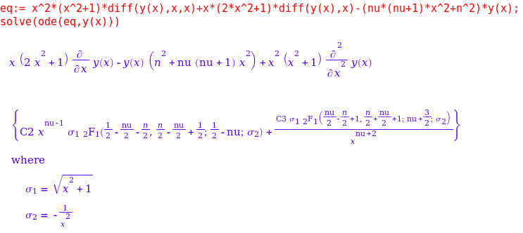
This is just a small selection of the enhancements that The Mathworks have made to the symbolic toolbox which is coming along in leaps and bounds in my humble opinion. Thanks to various members of staff at The Mathworks for supplying me with these examples (and a fair few more besides). I wouldn’t have been able to make this post without them.
Other articles on Walking Randomly about the symbolic toolbox for MATLAB:
- Review of the new symbolic toolbox in MATLAB 2008b (written just after the transfer from a Maple symbolic engine to the new Mupad one)
Changes to the Optimization toolbox
- The fmincon function now has a new algorithm available. The algorithm is called SQP which stands for Sequential Quadratic Programming. I don’t know much about it yet but may return to this in the future.
Licensing changes
Licensing and toolbox naming might be dull for most people – but it is a big deal to me since I work in a team that administers a large network license for MATLAB. Changes that might seem minor to most people can result in drastic improvements for the life of a network license administrator. On the other hand, some changes can result in massive amounts of work.
- Solaris as a network license platform was dropped. This is a shame because although my employer has very few Solaris client machines, it currently runs its MATLAB license server on Solaris and it has been (and continues to be) rock solid. Now we are going to have to move to Windows license servers and update every single client machine on campus before we can update to 2010a. Oh joys!
- The Genetic Algorithm and Direct Search toolbox is no more. It’s functionality is now part of the Global Optimization Toolbox. I’ve not used this one myself yet but it does have a small core set of users at my university.
Articles aimed at users of MATLAB network licenses include
- More MATLAB statistics toolbox licensing woes (and how to solve them)
- An alternative to binopdf using the NAG toolbox for MATLAB
Much of the fine detail in this article was provided to me by members of staff at The Mathworks. I thank them all for their time, patience and expertise in answering my incessant questions. Any mistakes, however, are my fault!
If you enjoyed this article, feel free to click here to subscribe to my RSS Feed.
A little while ago I was having a nice tea break when all hell broke loose. Complaint after complaint started rolling in about lack of network licenses for the MATLAB statistics toolbox and everyone was wondering what I intended to do about it. A quick look at our license server indicated that someone had started a large number of MATLAB jobs on a Beowulf cluster and all of them used the statistics toolbox. Slowly but surely, he was eating up every statistics toolbox license in the university.
I contacted him, explained the problem and he terminated all of his jobs. Life returned to normal for the rest of the university but now he couldn’t work. What to do?
One option was to compile his code using the MATLAB compiler and send the resulting binaries to the cluster but I took another route. I had a look through his code and discovered that he was only ever calling one function from the Statistics toolbox and that was
random('unif',0,1)
All this does is give a uniform random number between 0 and 1. However, if you code it like this
rand()
then you won’t use a license from the statistics toolbox since rand() is part of basic MATLAB. Of course most people don’t want a random number between 0 and 1; instead they will want a random number between two constants, a and b. In almost all cases the following two statements are mathematically equivalent
r = a + (b-a).*rand();     %Doesn't use a license for the statistics toolbox
r = random('unif',a,b);    %Does use a license for the statistics toolbox
The statistics toolbox function, random(), is much more general than rand() since it can give you random numbers from many different distributions but you are wasting a license token if you use it for the uniform distribution. The same goes for the normal distribution for that matter since basic MATLAB has randn().
random('norm',mu,sigma);  %does use a stats license
r = randn()* sigma + mu;  %doesn't use a stats license
The moral of the story is that when you are using MATLAB in a network licensed environment, it can sometimes pay to consider how you spell your functions ;)
According to a new website, if you plot the following equation
then you’ll get the following graph
Head over to the Inverse Graphing Calculator to generate your own. It would be interesting to solve these equations and see if the website is correct.
If you liked this post then you may like this one too: Secret messages hidden inside equations
One of MATLAB’s strengths is that it has a toolbox for almost everything. One of it’s weaknesses is that you have to pay separately for them all! Basic MATLAB is cheaper for most people than basic Mathematica but, in my experience at least, many people need access to statistics, optimization,symbolics, curve fitting and (increasingly) parallel toolboxes before they get functionality equivalent to Mathematica. By the time one has bought all of those additional toolboxes, MATLAB doesn’t look quite so cheap!
I am growing a list of quality, free MATLAB toolboxes and it is clear that the world could do with more. So, I have a question for you all. If you could have one MATLAB toolbox for free then which one would it be?
The Problem
A MATLAB user came to me with a complaint recently. He had a piece of code that made use of the MATLAB Statistics toolbox but couldn’t get reliable access to a stats toolbox license from my employer’s server. You see, although we have hundreds of licenses for MATLAB itself, we only have a few dozen licenses for the statistics toolbox. This has always served us well in the past but use of this particular toolbox is on the rise and so we sometimes run out which means that users are more likely to get the following error message these days
??? License checkout failed.
License Manager Error -4
Maximum number of users for Statistics_Toolbox reached.
Try again later.
To see a list of current users use the lmstat utility or contact your License Administrator.
The user had some options if he wanted to run his code via our shared network licenses for MATLAB (rather than rewrite in a free language or buy his own, personal license for MATLAB):
- Wait until a license became free.
- Wait until we found funds for more licenses.
- Buy an additional license token for himself and add it to the network (235 pounds +VAT currently)
- Allow me to gave a look at his code and come up with another way
He went for the final option. So, I sat with a colleague of mine and we looked through the code. It turned out that there was only one line in the entire program that used the Statistics toolbox and all that line did was call binopdf. That one function call almost cost him 235 quid!
Now, binopdf() simply evaluates the binomial probability density function and the definition doesn’t look too difficult so you may wonder why I didn’t just cook up my own version of binopdf for him? Quite simply, I don’t trust myself to do as good a job as The Mathworks. There’s bound to be gotchas and I am bound to not know them at first. What would you rather use, binpodf.m from Mathworks or binopdf.m from ‘Dodgy Sysadmin’s Functions Inc.’? Your research depends upon this function remember…
NAG to the rescue!
I wanted to use a version of this function that was written by someone I trust so my mind immediately turned to NAG (Numerical Algorithms Group) and their MATLAB toolbox which my employer has a full site license for. The NAG Toolbox for MATLAB has a function called g01bj which does what we need and a whole lot more. The basic syntax is
[plek, pgtk, peqk, ifail] = g01bj(n, p, x)
From the NAG documentation: Let X denote a random variable having a binomial distribution with parameters n and p. g01bj calculates the following probabilities
- plek = Prob{X<=x}
- pgtk = Prob{X > x}
- peqk = Prob{X = x}
MATLAB’s binopodf only calculates Prob(X=x) so the practical upshot is that for the following MATLAB code
n=200;
x=0;
p=0.02;
y=binopdf(x,n,p)
the corresponding NAG Toolbox code (on a 32bit machine) is
n=int32(200);
x=int32(0);
p=0.02;
[plek, pgtk, y, ifail] = g01bj(n, p, x);
both of these code snippets gives
y =
    0.0176
Further tests show that NAG’s and MATLAB’s results agree either exactly or to within what is essentially numerical noise for a range of values. The only thing that remained was to make NAG’s function look more ‘normal’ for the user in question which meant creating a file called nag_binopdf.m which contained the following
function pbin = nag_binopdf(x,n,p)
   x=int32(x);
   n=int32(n);
   [~,~,pbin,~] = g01bj(n,p,x);
end
Now the user had a function called nag_binopdf that behaved just like the Statistics toolbox’s binopdf, for his particular application, argument order and everything.
It’s not all plain sailing though!
As good as the NAG toolbox is, it’s not perfect. Note that I placed particular emphasis on the fact that we had come up with a suitable, drop-in replacement for binopdf for this user’s particular application. The salient points of his application are:
- His input argument, x, is just a single value – not a vector of values. The NAG library wasn’t written with MATLAB in mind, it’s written in Fortran, and so many of its functions are not vectorised (some of them are though). In Fortran this is no problem at all but in MATLAB it’s a pain. I could, of course, write a nag_binopodf that looks like it’s vectorised by putting g01bj in a loop hidden away from the user but I’d soon get found out because the performance would suck. To better support MATLAB users, NAG needs to write properly vectorised versions of its functions.
- He only wanted to run his code on 32bit machines. If he had wanted to run it on a 64bit machine then he would have to change all of those int32() calls to int64(). I agree that this is no big deal but it’s something that he wouldn’t have to worry about if he had coughed up the cash for a Mathworks statistics license.
Final thoughts
I use the NAG toolbox for MATLAB to do this sort of thing all the time and have saved researchers at my university several thousand pounds over the last year or so through unneeded Mathworks toolbox licenses. As well as statistics, the NAG toolbox is also good for optimisation (local and global), curve fitting, splines, wavelets, finance,partial differential equations and probably more. Not everyone likes this approach and it is not always suitable but when it works, it works well. Sometimes, you even get a significant speed boost into the bargain (check out my interp1 article for example).
Comments are, as always, welcomed.
Blog posts similar to this one