
Archive for April, 2010
I have got a nice, shiny 64bit version of MATLAB running on my nice, shiny 64bit Linux machine and so, naturally, I wanted to be able to use 64 bit integers when the need arose. Sadly, MATLAB had other ideas. On MATLAB 2010a:
a=int64(10);
b=int64(20);
a+b
??? Undefined function or method 'plus' for input arguments of type 'int64'.
It doesn’t like any of the other operators either
>> a-b
??? Undefined function or method 'minus' for input arguments of type 'int64'.

>> a*b
??? Undefined function or method 'mtimes' for input arguments of type 'int64'.

>> a/b
??? Undefined function or method 'mrdivide' for input arguments of type 'int64'.
At first I thought that there was something wrong with my MATLAB installation but it turns out that this behaviour is expected and documented. At the time of writing, the MATLAB documentation contains the lines
Note   Only the lower order integer data types support math operations.
Math operations are not supported for int64 and uint64.
So, there you have it. When can’t MATLAB add up? When you ask it to add 64 bit integers!
Update: Just had an email from someone who points out that Octave (Free MATLAB Clone) can handle 64bit integers just fine
octave:1> a=int64(10);
octave:2> b=int64(20);
octave:3> a+b
ans = 30
octave:4>
Update 2: Since I got slashdotted, people have been asking why I (or, more importantly, the user I was helping) needed 64bit integers. Well, we were using the NAG Toolbox for MATLAB which is a MATLAB interface to the NAG Fortran library. Some of its routines require integer arguments and on a 64bit machine these must be 64bit integers. We just needed to do some basic arithmetic on them before passing them to the toolbox and discovered that we couldn’t. The work-around was simple – use int32s for the arithmetic and then convert to int64 at the end so no big deal really. I was simply surprised that arithmetic wasn’t supported for int64s directly – hence this post.
Update 3: In the comments, someone pointed out that there is a package on the File Exchange that adds basic arithmetic support for 64bit integers. I’ve not tried it myself though so can’t comment on its quality.
Update 4: Someone has made me aware of an interesting discussion concerning this topic on MATLAB Central a few years back: http://www.mathworks.com/matlabcentral/newsreader/view_thread/154955
Update 5 (14th September 2010): MATLAB 2010b now has support for 64 bit integers.
Late last year I was asked to give a talk at my University to a group of academics studying financial mathematics (Black-Scholes, monte-carlo simulations, time series analysis – that sort of thing). The talk was about the NAG Numerical Library, what it could do, what environments you can use it from, licensing and how they could get their hands on it via our site license.
I also spent a few minutes talking about Python including why I thought it was a good language for numerical computing and how to interface it with the NAG C library using my tutorials and PyNAG code. I finished off with a simple graphical demonstration that minimised the Rosenbrock function using Python, Matplotlib and the NAG C-library running on Ubuntu Linux.
“So!”, I asked, “Any questions?”
The very first reply was “Does your Python-NAG interface work on Windows machines?” to which the answer at the time was “No!” I took the opportunity to ask the audience how many of them did their numerical computing in Windows (Most of the room of around 50+ people), how many people did it using Mac OS X (A small group at the back), and how many people did it in Linux (about 3).
So, if I wanted the majority of that audience to use PyNAG then I had to get it working on Windows. Fortunately, thanks to the portability of Python and the consistency of the NAG library across platforms, this proved to be rather easy to do and the result is now available for download on the main PyNAG webpage.
Let’s look at the main differences between the Linux and Windows versions
Loading the NAG Library
In the examples given in my Linux NAG-Python tutorials, the cllux08dgl NAG C-library was loaded using the line
libnag = cdll.LoadLibrary("/opt/NAG/cllux08dgl/lib/libnagc_nag.so.8")
In Windows the call is slightly different. Here it is for CLDLL084ZL (Mark 8 of the C library for Windows)
C_libnag = ctypes.windll.CLDLL084Z_mkl
If you are modifying any of the codes shown in my NAG-Python tutorials then you’ll need to change this line yourself. If you are using PyNAG, however, then it will already be done for you.
Callback functions
For my full introduction to NAG callback functions on Linux click here. The main difference between using callbacks on Windows compared to Linux is that on Linux we have
C_FUNC = CFUNCTYPE(c_double,c_double )
but on Windows we have
C_FUNC = WINFUNCTYPE(c_double,c_double )
There are several callback examples in the PyNAG distribution.
That’s pretty much it I think. Working through all of the PyNAG examples and making sure that they ran on Windows uncovered one or two bugs in my codes that didn’t affect Linux for one reason or another so it was a useful exercise all in all.
So, now you head over to the main PyNAG page and download the Windows version of my Python/NAG interface which includes a set of example codes. I also took the opportunity to throw in a couple of extra features and so upgraded PyNAG to version 0.16, check out the readme for more details. Thanks to several employees at NAG for all of their help with this including Matt, John, David, Marcin and Sorin.
I work for the University of Manchester in the UK as a ‘Science and Engineering Applications specialist’ which basically means that I am obsessed with software used by mathematicians and scientists. One of the applications within my portfolio is the NAG library – a product that we use rather a lot in its various incarnations. We have people using it from Fortran, C, C++, MATLAB, Python and even Visual Basic in areas as diverse as engineering, applied maths, biology and economics.
Yes, we are big users of NAG at Manchester but then that stands to reason because NAG and Manchester have a collaborative history stretching back 40 years to NAG’s very inception. Manchester takes a lot of NAG’s products but for reasons that are lost in the mists of time, we have never (to my knowledge at least) had a site license for their SMP library (more recently called The NAG Library for SMP & multicore). Very recently, that changed!
SMP stands for Symmetric Multi-Processor which essentially means ‘two or more CPUs sharing the same bit of memory.’ Five years ago, it would have been rare for a desktop user to have an SMP machine but these days they are everywhere. Got a dual-core laptop or a quad-core desktop? If the answer’s ‘yes’ then you have an SMP machine and you are probably wondering how to get the most out of it.
‘How can I use all my cores (without any effort)’
One of the most common newbie questions I get asked these days goes along the lines of ‘Program X is only using 50%/25%/12.5% of my CPU – how can I fix this?’ and, of course, the reason for this is that the program in question is only using a single core of their multicore machine. So, the problem is easy enough to explain but not so easy to fix because it invariably involves telling the user that they are going to have to learn how to program in parallel.
Explicit parallel programming is a funny thing in that sometimes it is trivial and other times it is pretty much impossible – it all depends on the problem you see. Sometimes all you need to do is drop a few OpenMP pragmas here and there and you’ll get a 2-4 times speed up. Other times you need to completely rewrite your algorithm from the ground up to get even a modest speed up. Yet more times you are simply stuck because your problem is inherently non-parallelisable. It is even possible to slow your code down by trying to parallelize it!
If you are lucky, however, then you can make use of all those extra cores with no extra effort at all! Slowly but surely, mathematical software vendors have been re-writing some of their functions to ensure that they work efficiently on parallel processors in such a way that it is transparent to the user. This is sometimes referred to as implicit parallelism.
Take MATLAB, for example, ever since release 2007a more and more built in MATLAB functions have been modified to allow them to make full use of multi-processor systems. If your program makes extensive use of these functions then you don’t need to spend extra money or time on the parallel computing toolbox, just run your code on the latest version of MATLAB, sit back and enjoy the speed boost. It doesn’t work for all functions of course but it does for an ever increasing subset.
The NAG SMP Library – zero effort parallel programming
For users of NAG routines, the zero-effort approach to making better use of your multicore system is to use their SMP library. According to NAG’s advertising blurb you don’t need to rewrite your code to get a speed boost – you just need to link to the SMP library instead of the Fortran library at compile time.
Just like MATLAB, you won’t get this speed boost for every function, but you will get it for a significant subset of the library (around 300+ functions as of Mark 22 – the full list is available on NAG’s website). Also, just like MATLAB, sometimes the speed-up will be massive and other times it will be much more modest.
I wanted to test NAG’s claims for myself on the kind of calculations that researchers at Manchester tend to perform so I asked NAG for a trial of the upcoming Mark 22 of the SMP library and, since I am lazy, I also asked them to provide me with simple demonstration programs and I’d like to share the results with you all. These are not meant to be an exhaustive set of benchmarks (I don’t have the time to do such a thing) but should give you an idea of what you can expect from NAG’s new library.
System specs
All of these timings were made on a 3Ghz Intel Core2 Quad Q9650 CPU desktop machine with 8Gb of RAM running Ubuntu 9.10. The serial version of the NAG library used was fll6a22dfl and the SMP version of the library was fsl6a22dfl. The version of gfortran used was 4.4.1 and the cpu-frequency governor was switched off as per a previous blog post of mine.
Example 1 – Nearest correlation matrix
The first routine I looked at was one that calculated the nearest correlation matrix. In other words ‘Given a symmetric matrix, what is the nearest correlation matrix—that is, the nearest symmetric positive semidefinite matrix with unit diagonal?’[1] This is a problem that pops up a lot in Finance – option pricing, risk management – that sort of thing.
The NAG routine that calculates the nearest correlation matrix is G02AAF which is based on the algorithm developed by Qi and Sun[2]. The example program I was sent first constructs a N x N tridiagonal matrix A of the form A(j,j)=2, A(j-1,j)=-1.1 and A(j,j-1)=1.0. It then times how long it takes G02AAF to find the nearest correlation matrix to A. You can download this example, along with all supporting files, from the links below.
To compile this benchmark against the serial library I did
gfortran ./bench_g02aaf.f90 shtim.c wltime.f /opt/NAG/fll6a22dfl/lib/libnag_nag.a  \
/opt/NAG/fll6a22dfl/acml/libacml_mv.a -o serial_g02aaf
To compile the parallel version I did
gfortran -fopenmp ./bench_g02aaf.f90 shtim.c wltime.f /opt/NAG/fsl6a22dfl/lib/libnagsmp.a \
  /opt/NAG/fsl6a22dfl/acml4.3.0/lib/libacml_mp.a -o smp_g02aaf
I didn’t need to modify the source code in any way when going from a serial version to a parallel version of this benchmark. The only work required was to link to the SMP library instead of the serial library – so far so good. Let’s run the two versions and see the speed differences.
First things first, let’s ensure that there is no limit to the stack size of my shell by doing the following in bash
ulimit -s unlimited
Also, for the parallel version, I need to set the number of threads to equal the number of processors I have on my machine by setting the OMP_NUM_THREADS environment variable.
export OMP_NUM_THREADS=4
This won’t affect the serial version at all. So, onto the program itself. When you run it, it will ask you for two inputs – an integer, N, and a boolean, IO. N gives the size of the starting matrix and IO determines whether or not to output the result.
Here’s an example run of the serial version with N=1000 and IO set to False. (In Fortran True is represented as .t. and False is represented as .f. )
./serial_g02aaf
 G02AAF: Enter N, IO
1000 .f.
 G02AAF: Time, IFAIL =    37.138997077941895                0
 G02AAF: ITER, FEVAL, NRMGRD =            4           5  4.31049822255544465E-012
The only output I am really interested in here is the time and 37.13 seconds doesn’t seem too bad for a 1000 x 1000 matrix at first glance. Move to the parallel version though and you get a very nice surprise
./smp_g02aaf
 G02AAF: Enter N, IO
1000 .f.
 G02AAF: Time, IFAIL =    5.1906139850616455                0
 G02AAF: ITER, FEVAL, NRMGRD =            4           5  4.30898281428799420E-012
The above times were typical and varied little from run to run (although the SMP version varied by a bigger percentage than the serial version). However I averaged over 10 runs to make sure and got 37.14 s for the serial version and 4.88 s for the SMP version which gives a speedup of 7.6 times!
Now, this is rather impressive. Usually, when one parallelises over N cores then the very best you can expect in an ideal word is a speed up of just less than N times, so called ‘linear scaling’. Here we have N=4 and a speedup of 7.6 implying that NAG have achieved ‘super-linear scaling’ which is usually pretty rare.
I dropped them a line to ask what was going on. It turns out that when they looked at parallelising this routine they worked out a way of speeding up the serial version as well. This serial speedup will be included in the serial library in its next release, Mark 23 but the SMP library got it as of Mark 22.
So, some of that 7.6 times speedup is as a result of serial speedup and the rest is parallelisation. By setting OMP_NUM_THREADS to 1 we can force the SMP version of the benchmark to only run on only one core and thus see how much of the speedup we can attribute to parallelisation:
export OMP_NUM_THREADS=1
./smp_g02aaf
 G02AAF: Enter N, IO
1000 .f.
 G02AAF: Time, IFAIL =    12.714214086532593                0
 G02AAF: ITER, FEVAL, NRMGRD =            4           5  4.31152424170390294E-012
Recall that the 4 core version took an average of 4.88 seconds so the speedup from parallelisation alone is 2.6 times – much closer to what I expected to see. Now, it is probably worth mentioning that there is an extra level of complication (with parallel programming there is always an extra level of complication) in that some of this parallelisation speedup comes from extra work that NAG has done in their algorithm and some of it comes from the fact that they are linking to parallel versions of the BLAS and LAPACK libraries. We could go one step further and determine how much of the speed up comes from NAG’s work and how much comes from using parallel BLAS/LAPACK but, well, life is short.
The practical upshot is that if you come straight from the Mark 22 serial version then you can expect a speed-up of around 7.6 times. In the future, when you compare the Mark 22 SMP library to the Mark 23 serial library then you can expect a speedup of around 2.6 times on a 4 core machine like mine.
Example 2 – Quasi random number generation
Quasi random numbers (also referred to as ‘Low discrepancy sequences’) are extensively used in Monte-Carlo simulations which have applications in areas such as finance, chemistry and computational physics. When people need a set of quasi random numbers they usually need a LOT of them and so the faster they can be produced the better. The NAG library contains several quasi random number generators but the one considered here is the routine g05ymf. The benchmark program I used is called bench_g05ymf.f90 and the full set of files needed to compile it are available at the end of this section.
The benchmark program requires the user to input 4 numbers and a boolean as follows.
- The first number is the quasi random number generator to use with the options being:
- NAG’s newer Sobol generator (based on the 2008 Joe and Kuo algorithm[3] )
- NAG’s older Sobol generator
- NAG’s Niederreiter generator
- NAG’s Faure generator
- The second number is the order in which the generated values are returned (The parameter RCORD as referred to in the documentation for g05ymf). Say that the matrix of returned values is called QUAS then if RCORD=1, QUAS(i,j) holds the jth value for the ith dimension, otherwise QUAS(i,j) holds the ith value for the jth dimension.
- The third number is the number of dimensions required.
- The fourth number is the number of number of quasi-random numbers required.
- The boolean (either .t. or .f.) determines whether or not the output should be verbose or not. A value of .t. will output the first 100 numbers in the sequence.
To compile the benchmark program against the serial library I did:
gfortran ./bench_g05ymf.f90 shtim.c wltime.f /opt/NAG/fll6a22dfl/lib/libnag_nag.a  \
/opt/NAG/fll6a22dfl/acml/libacml_mv.a -o serial_g02aaf
As before, the only thing needed to turn this into a parallel program was to compile against the SMP library and add the -fopenmp switch
gfortran -fopenmp ./bench_g05ymf.f90 shtim.c wltime.f /opt/NAG/fsl6a22dfl/lib/libnagsmp.a  \
/opt/NAG/fsl6a22dfl/acml4.3.0/lib/libacml_mp.a -o smp_g02aaf
The first set of parameters I used was
1 2 900 1000000 .f.
Which uses NAG’s new Sobol generator with RCORD=2 to generate and store 1,000,000 numbers over 900 dimensions with no verbose output. Averaged over 10 runs the times were 5.17 seconds for the serial version and 2.14 seconds for the parallel version giving a speedup of 2.4x on a quad-core machine. I couldn’t push number of dimensions much higher because the benchmark stores all of the numbers in one large array and I was starting to run out of memory.
If you only want a relatively small sequence then switching to the SMP library is actually slower thanks to the overhead involved in spawning extra threads. For example if you only want 100,000 numbers over 8 dimensions:
1 2 8 100000 .f.
then the serial version of the code takes an average of 0.0048 seconds compared to 0.0479 seconds for the parallel version so the parallel version is almost 10 times slower when using 4 threads for small problems. Setting OMP_NUM_THREADS to 1 gives exactly the same speed as the serial version as you might expect.
NAG have clearly optimized this function to ensure that you get a good speedup for large problem sets which is where it really matters so I am very pleased with it. However, the degradation in performance for smaller problems concerns me a little. I think I’d prefer it if NAG were to modify this function so that it works serially for small sequences and to automatically switch to parallel execution if the user requests a large sequence.
Conclusions
In the old days we could speedup our programs simply by buying a new computer. The new computer would have a faster clock speed than the old one and so our code would run faster with close to zero effort on our part. Thanks to the fact that clock speeds have stayed more or less constant for the last few years those days are over. Now, when we buy a new computer we get more processors rather than faster ones and this requires a change in thinking. Products such as the NAG Library for SMP & multicore help us to to get the maximum benefit out of our machines with the minimum amount of effort on our part. If switching to a product like this doesn’t give you the performance boost you need then the next thing for you to do is to learn how to program in parallel. The free ride is over.
In summary:
- You don’t need to modify your code if it already uses NAG’s serial library. Just recompile against the new library and away you go. You don’t need to know anything about parallel programming to make use of this product.
- The SMP Library works best with big problems. Small problems don’t work so well because of the inherent overheads of parallelisation.
- On a quad-core machine you can expect speed-ups around 2-4 times compared to the serial library. In exceptional circumstances you can expect speed-up as large as 7 times or more.
- You should notice a speed increase in over 300 functions compared to the serial library.
- Some of this speed increase comes from fundamental libraries such as BLAS and LAPACK, some of it comes from NAG directly parallelising their algorithms and yet more comes from improvements to the underlying serial code.
- I’m hoping that this Fortran version is just the beginning. I’ve always felt that NAG program in Fortran so I don’t have to and I’m hoping that they will go on to incorporate their SMP improvements in their other products, especially their C library and MATLAB toolbox.
Acknowledgements
Thanks to several staff at NAG who suffered my seemingly endless stream of emails during the writing of this article. Ed, in particular, has the patience of a saint. Any mistakes left over are all mine!
Links
- The Nearest Correlation Matrix benchmark program used here – bench_g02aaf.f90 – along with the source code for the timing routine.
- NAG’s documentation for the g02aaf routine.
- The Quasi Random Number benchmark program used here – bench_g05ymf.f90 – along with the source code for the timing routine.
- An Introduction to quasi random numbers (written by a member of NAG’s staff)
- Official NAG documentation for g05ymf – the quasi random number generator considered here.
References
[1] – Higham N, Computing the nearest correlation matrix—a problem from finance, IMA Journal of Numerical Analysis 22 (3): 329–343
[2] – Qi H and Sun D (2006), A Quadratically Convergent Newton Method for Computing the Nearest
Correlation Matrix, SIAM J. Matrix AnalAppl 29(2) 360–385
[3] – Joe S and Kuo F Y (2008) Constructing Sobol sequences with better two-dimensional projects SIAM J. Sci. Comput. 30 2635–2654
Dislaimer: This is a personal blog and the opinions expressed on it are mine and do not necessarily reflect the policies and opinions of my employer, The University of Manchester.
I was recently playing with some parallel code that used gfortran and OpenMP to parallelise a calculation over 4 threads and was getting some seriously odd timing results. The first time I ran the code it completed in 4.8 seconds, the next run took 4.8 seconds but the third run took 84 seconds (No, I haven’t missed off the decimal point). Subsequent timings were all over the place – 12 seconds, 4.8 seconds again, 14 seconds….something weird was going on.
I wouldn’t mind but all of these calculations had exactly the same input/output and yet sometimes this parallel code took significantly longer to execute than the serial version.
On drilling down I discovered that two of the threads had 100% CPU utilisation and the other two only had 50%. On a hunch I wondered if the CPU frequency ‘on demand’ scaling thing was messing things (It has done so in the past) up so I did
sudo cpufreq-selector -c 0 -f 3000
sudo cpufreq-selector -c 1 -f 3000
sudo cpufreq-selector -c 2 -f 3000
sudo cpufreq-selector -c 3 -f 3000
to set the cpu-frequency of all 4 cores to the maxium 3Ghz. This switched off the ‘on demand’ setting that is standard in Ubuntu.
Lo! it worked! 4.8 seconds every time. When I turned the governor back on
sudo cpufreq-selector --governor ondemand
I got back the ‘sometimes it’s fast, sometimes it’s slow’ behaviour. Oddly, one week and several reboots later I can’t get back the slow behaviour no matter what I set the governor to.
Perhaps this was just a temporary glitch in my system but, as I said earlier, I have seen this sort of behaviour before so, just to be on the safe side, it might be worth switching off the automatic governor whenever you do parallel calculations in Linux.
Does anyone have any insight into this? Comments welcomed.
I’ve been following the progress of Mathcad Prime, the upcoming replacement for PTC’s Mathcad, for a few months now and have managed to get my hands on a few preview screen shots. Click on each image to obtain a full resolution version

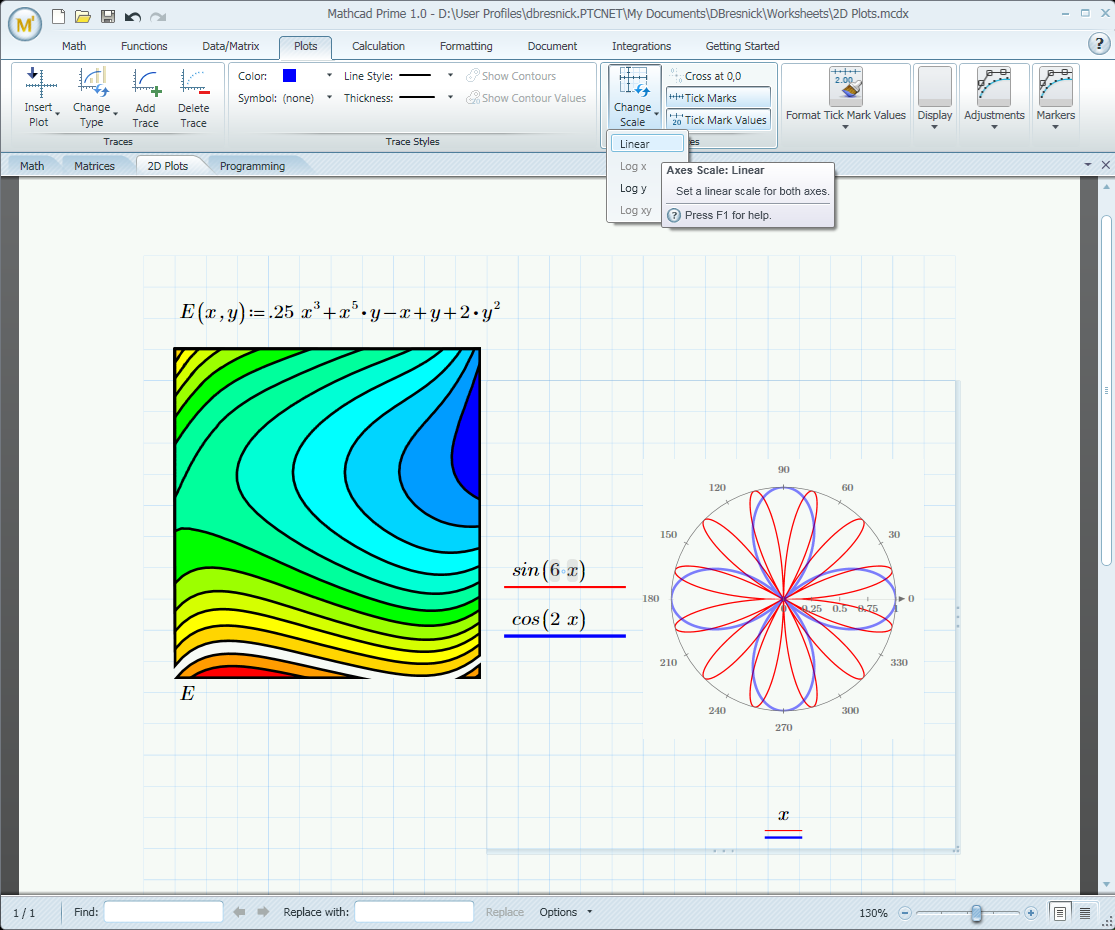
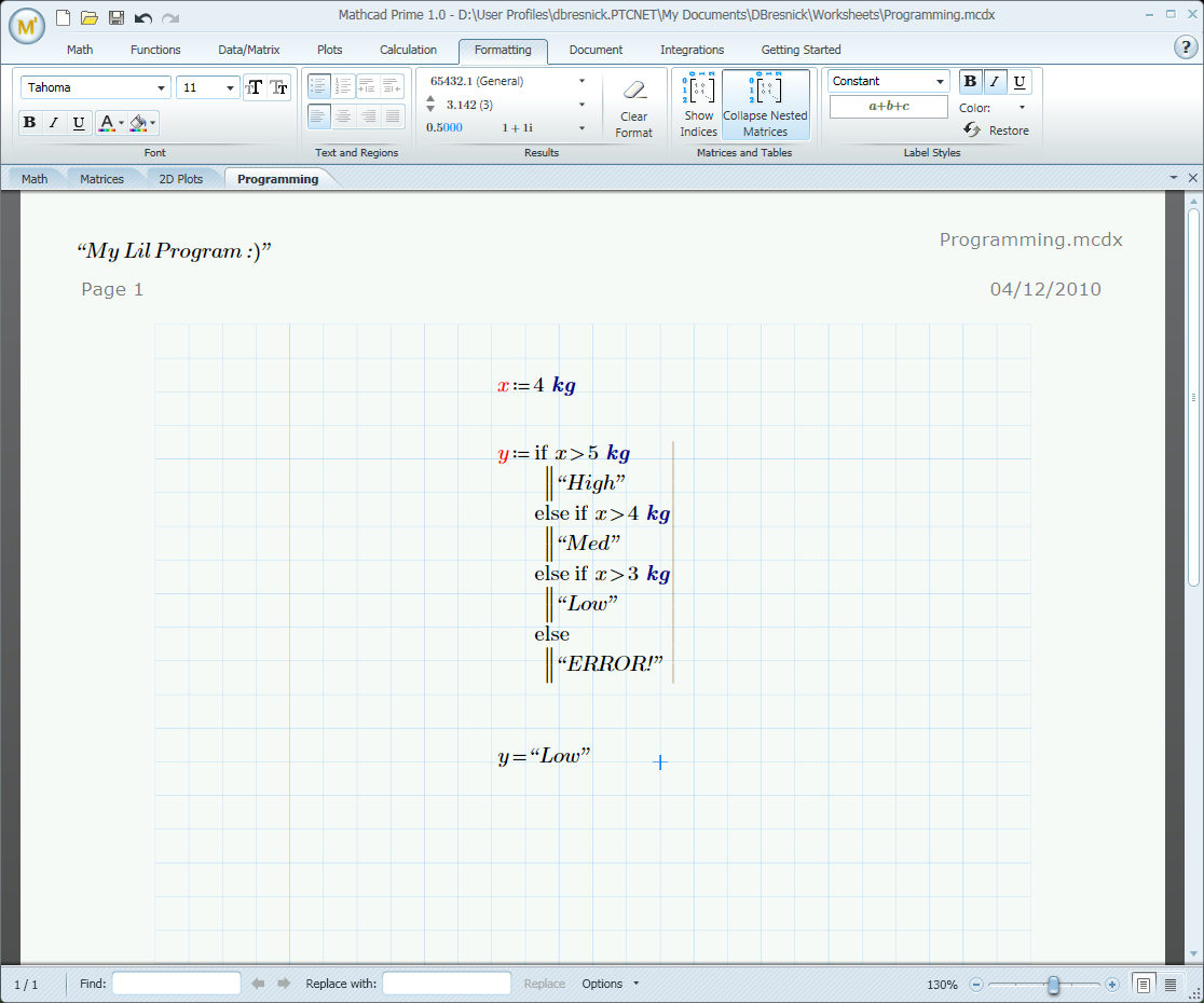
I’m particularly pleased to see that final image since it demonstrates that Mathcad Prime will support programming constructs. There were rumours a while ago that Prime would not be capable of either symbolics or programming which concerned me somewhat because I support users that require both.
A couple of weeks ago, PTC arranged a virtual conference where a couple of PTC developers demonstrated the latest build of Mathcad Prime. The focus was very much on Prime’s ease of use and its ability to handle units and I have to say I was impressed – it seems to be a big improvement over Mathcad 14. As long as symbolics makes it into Prime then I think I am going to be rather happy with it.
It is still possible to check out the recordings of the virtual conference yourself at http://events.unisfair.com/index.jsp?eid=522&seid=25 (requires registration). If you’ve seen the presentation then I’d love to know what you think so drop me a comment and say hi.
A shameless copy of The Endeavour’s weekend miscellany
Programming
- A Mathematica package for accessing Flikr – doing some cool stuff with Mathematica’s image processing commands.
Food
- What looks like a strawberry, but is white and tastes like a pineapple? – Tasty and weird looking. What more do you want from your food?
- Beef stew – recipe from TV chef Jamie Oliver. I’ve cooked this loads of times now and it never lets me down.
Technology
- First Ipad Reviews are in – Makes me want one more
Life
- Philip Pullman’s Riposte – Damn right!
- Simon Singh wins libel court battle – Common sense prevails at last.
- Animals living without oxygen found – Proving that life is tougher than we thought.
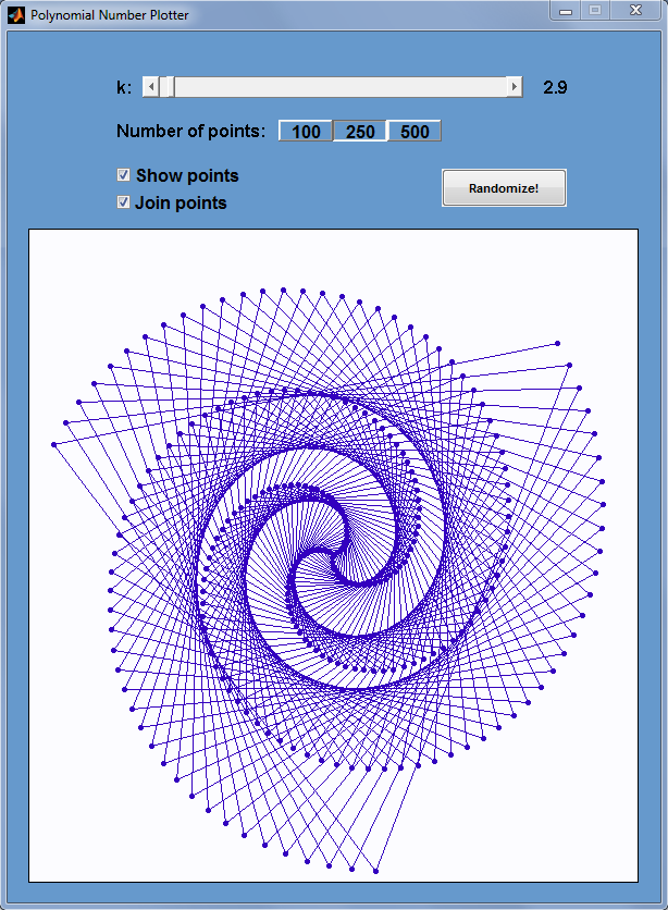
After reading my recent post, Polygonal numbers on quadratic number spirals, Walking Randomly reader Matt Tearle came up with a MATLAB version and it looks great. Click on the image below for the code.
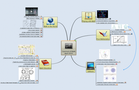
The 64th Carnival of mathematics has been posted over at Maria’s Teaching College Math blog and it is rather different from the norm. Posted as a mind map, it includes articles on a Murder Mystery project for logarithms, weightlifting for the brain, MATLAB, R, the mathematics behind a good night’s sleep and much more.
If you are new to math carnivals and are wondering what is going on then check out my introductory post here.
Other recent carnivals include:
- Math Teachers at Play #24 – posted at Let’s play Math
- Carnival of maths #63 – posted at Mathrecreation
- Math Teachers at Play #23 – posted at Mathrecreation
- Carnival of maths #62 – posted at The Endeavour
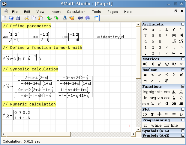
Andrey Ivashov’s free Mathcad alternative for Windows, Linux and Windows Mobile has recently been updated to version 0.87.3728 beta. This is a significant new release for SMath studio since this beta version adds support for units – possibly one of the most requested features on Andrey’s user forums.
I last looked at SMath Studio back in September 2009 and Andrey has made a lot of progress since then. As well as adding support for units and fixing some bugs he has added a whole host of user interface improvements including
- Dynamic assistance – SMath Studio can now be set to give you syntax hints and tips as you type your code.
- Support for plugins – Now we can all write something for SMath Studio
- A much smoother looking user interface – SMath Studio now looks much more professional than before
This fantastic free alternative to Mathcad is going from strength to strength and I am really enjoying watching its progress. Andrey has produced something that is genuinely useful, multiplatform, fun to use and, most importantly of all, he listens to his users. Well worth a download.