
Archive for the ‘math software’ Category
The MATLAB community site, MATLAB Central, is celebrating its 20th anniversary with a coding competition where the only aim is to make an interesting image with under 280 characters of code. The 280 character limit ensures that the resulting code is tweetable. There are a couple of things I really like about the format of this competition, other than the obvious fact that the only aim is to make something pretty!
- No MATLAB license is required! Sign up for a free MathWorks account and away you go. You can edit and run code in the browser.
Stealingreusing other people’s code is actively encouraged! The competition calls it remixing but GitHub users will recognize it as forking.
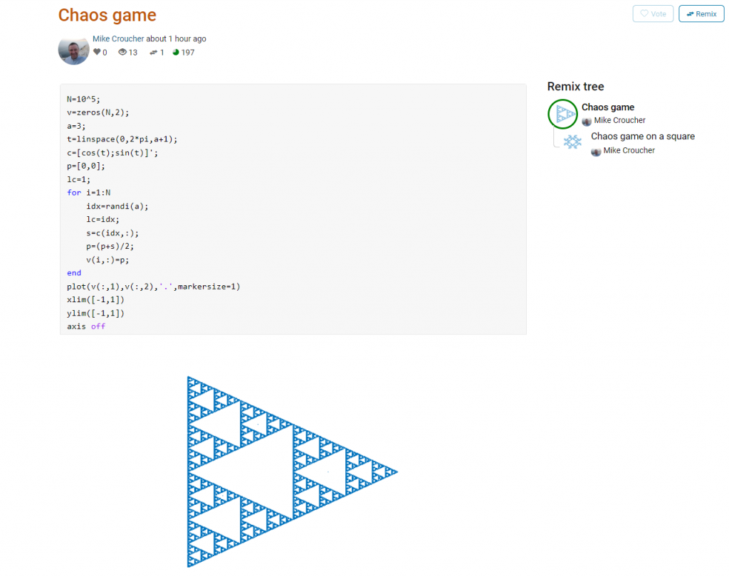
Here’s an example. I wrote a piece of code to render the Sierpiński triangle – Wikipedia using a simple random algorithm called the Chaos game.
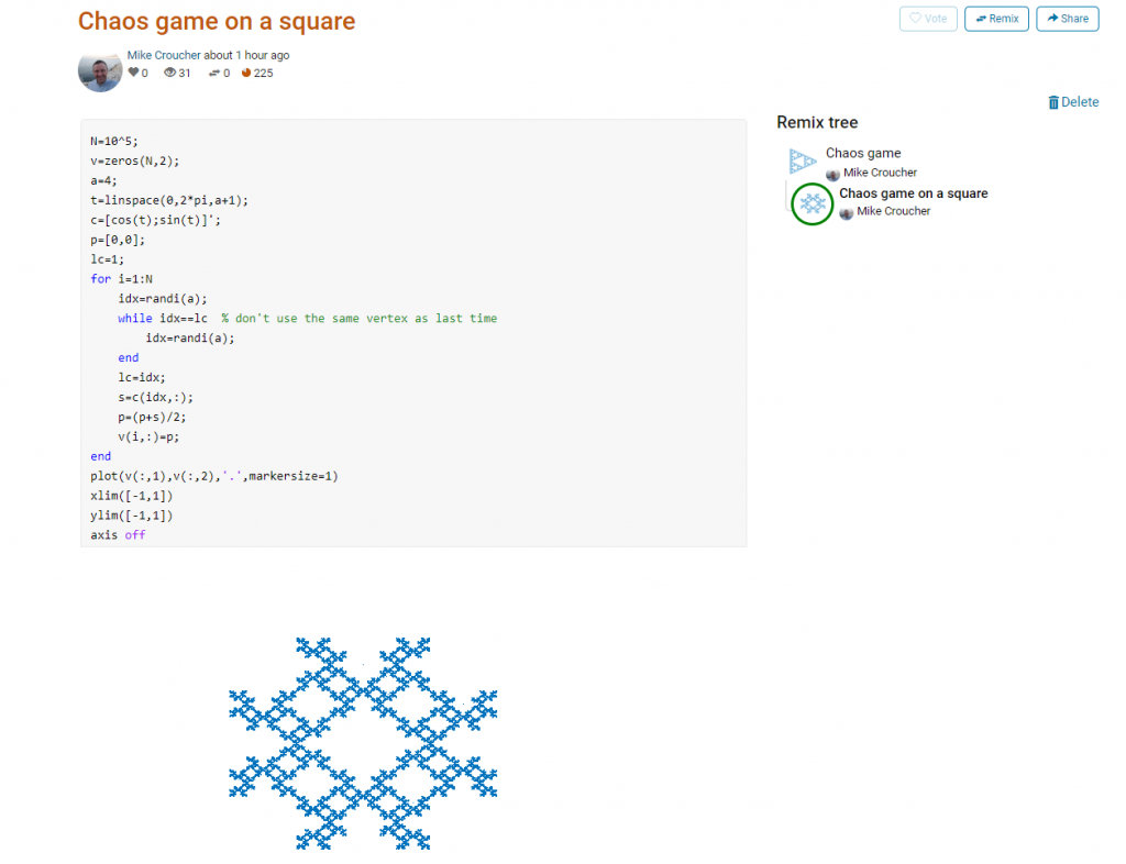
This is about as simple as the Chaos game gets and there are many things that could be done to produce a different image. As you can see from the Remix tree on the right hand side, I’ve already done one of them by changing a from 3 to 4 and adding some extra code to ensure that the same vertex doesn’t get chosen twice. This is result:
Someone else can now come along, hit the remix button and edit the code to produce something different again. Some things you might want to try for the chaos game include
- Try changing the value of a which is used in the variables t and c to produce the vertices of a polygon on an enclosing circle.
- Instead of just using the vertices of a polygon, try using the midpoints or another scheme for producing the attractor points completely.
- Try changing the scaling factor — currently p=(p+s)/2;
- Try putting limitations on which vertex is chosen. This remix ensures that the current vertex is different from the last one chosen.
- Each vertex is currently equally likely to be chosen using the code idx=randi(a); Think of ways to change the probabilities.
- Think of ways to colorize the plots.
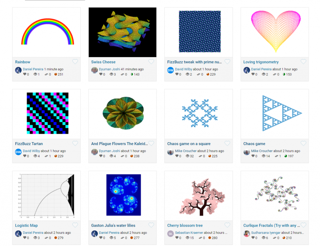
Maybe the chaos game isn’t your thing. You are free to create your own design from scratch or perhaps you’d prefer to remix some of the other designs in the gallery.
The competition is just a few hours old and there are already some very nice ideas coming out.
My stepchildren are pretty good at mathematics for their age and have recently learned about Pythagora’s theorem
$c=\sqrt{a^2+b^2}$
The fact that they have learned about this so early in their mathematical lives is testament to its importance. Pythagoras is everywhere in computational science and it may well be the case that you’ll need to compute the hypotenuse to a triangle some day.
Fortunately for you, this important computation is implemented in every computational environment I can think of!
It’s almost always called hypot so it will be easy to find.
Here it is in action using Python’s numpy module
import numpy as np
a = 3
b = 4
np.hypot(3,4)

5
When I’m out and about giving talks and tutorials about Research Software Engineering, High Performance Computing and so on, I often get the chance to mention the hypot function and it turns out that fewer people know about this routine than you might expect.
Trivial Calculation? Do it Yourself!
Such a trivial calculation, so easy to code up yourself! Here’s a one-line implementation
def mike_hypot(a,b):
    return(np.sqrt(a*a+b*b))
In use it looks fine
mike_hypot(3,4)

5.0
Overflow and Underflow
I could probably work for quite some time before I found that my implementation was flawed in several places. Here’s one
mike_hypot(1e154,1e154)

inf
You would, of course, expect the result to be large but not infinity. Numpy doesn’t have this problem
np.hypot(1e154,1e154)

1.414213562373095e+154
My function also doesn’t do well when things are small.
a = mike_hypot(1e-200,1e-200)

0.0
but again, the more carefully implemented hypot function in numpy does fine.
np.hypot(1e-200,1e-200)

1.414213562373095e-200
Standards Compliance
Next up — standards compliance. It turns out that there is a an official standard for how hypot implementations should behave in certain edge cases. The IEEE-754 standard for floating point arithmetic has something to say about how any implementation of hypot handles NaNs (Not a Number) and inf (Infinity).
It states that any implementation of hypot should behave as follows (Here’s a human readable summary https://www.agner.org/optimize/nan_propagation.pdf)
hypot(nan,inf) = hypot(inf,nan) = inf
numpy behaves well!
np.hypot(np.nan,np.inf)

inf

np.hypot(np.inf,np.nan)

inf
My implementation does not
mike_hypot(np.inf,np.nan)

nan
So in summary, my implementation is
- Wrong for very large numbers
- Wrong for very small numbers
- Not standards compliant
That’s a lot of mistakes for one line of code! Of course, we can do better with a small number of extra lines of code as John D Cook demonstrates in the blog post What’s so hard about finding a hypotenuse?
Hypot implementations in production
Production versions of the hypot function, however, are much more complex than you might imagine. The source code for the implementation used in openlibm (used by Julia for example) was 132 lines long last time I checked. Here’s a screenshot of part of the implementation I saw for prosterity. At the time of writing the code is at https://github.com/JuliaMath/openlibm/blob/master/src/e_hypot.c
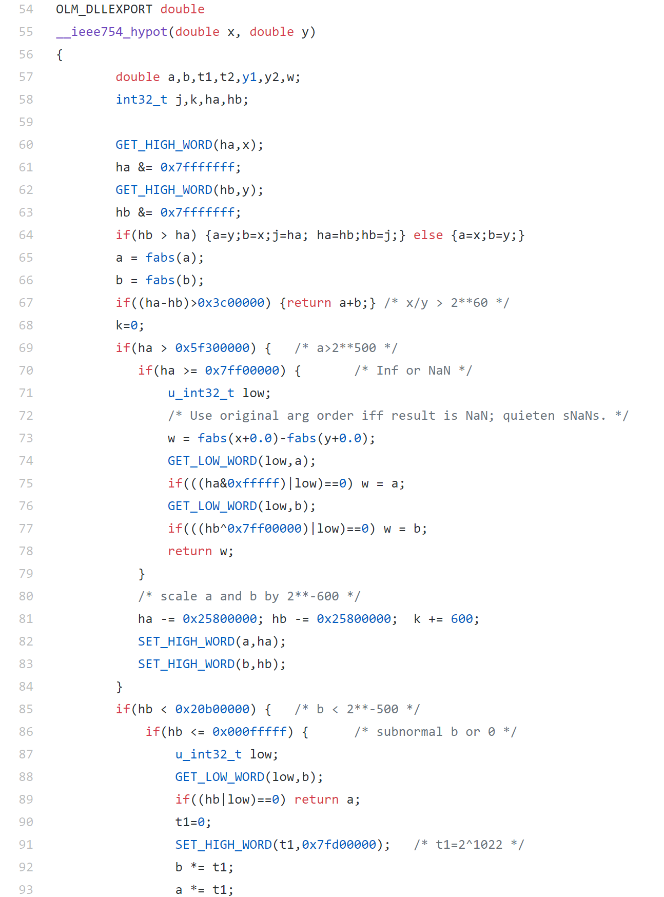
That’s what bullet-proof, bug checked, has been compiled on every platform you can imagine and survived code looks like.
There’s more!
Active Research
When I learned how complex production versions of hypot could be, I shouted out about it on twitter and learned that the story of hypot was far from over!
The implementation of the hypot function is still a matter of active research! See the paper here https://arxiv.org/abs/1904.09481

Is Your Research Software Correct?
Given that such a ‘simple’ computation is so complicated to implement well, consider your own code and ask Is Your Research Software Correct?.
What is Second Order Cone Programming (SOCP)?
Second Order Cone Programming (SOCP) problems are a type of optimisation problem that have applications in many areas of science, finance and engineering. A summary of the type of problems that can make use of SOCP, including things as diverse as designing antenna arrays, finite impulse response (FIR) filters and structural equilibrium problems can be found in the paper ‘Applications of Second Order Cone Programming’ by Lobo et al. There are also a couple of examples of using SOCP for portfolio optimisation in the GitHub repository of the Numerical Algorithms Group (NAG).
A large scale SOCP solver was one of the highlights of the Mark 27 release of the NAG library (See here for a poster about its performance). Those who have used the NAG library for years will expect this solver to have interfaces in Fortran and C and, of course, they are there. In addition to this is the fact that Mark 27 of the NAG Library for Python was released at the same time as the Fortran and C interfaces which reflects the importance of Python in today’s numerical computing landscape.
Here’s a quick demo of how the new SOCP solver works in Python. The code is based on a notebook in NAG’s PythonExamples GitHub repository.
NAG’s handle_solve_socp_ipm function (also known as e04pt) is a solver from the NAG optimization modelling suite for large-scale second-order cone programming (SOCP) problems based on an interior point method (IPM).
$$
\begin{array}{ll}
{\underset{x \in \mathbb{R}^{n}}{minimize}\ } & {c^{T}x} \\
\text{subject to} & {l_{A} \leq Ax \leq u_{A}\text{,}} \\
& {l_{x} \leq x \leq u_{x}\text{,}} \\
& {x \in \mathcal{K}\text{,}} \\
\end{array}
$$
where $\mathcal{K} = \mathcal{K}^{n_{1}} \times \cdots \times \mathcal{K}^{n_{r}} \times \mathbb{R}^{n_{l}}$ is a Cartesian product of quadratic (second-order type) cones and $n_{l}$-dimensional real space, and $n = \sum_{i = 1}^{r}n_{i} + n_{l}$ is the number of decision variables. Here $c$, $x$, $l_x$ and $u_x$ are $n$-dimensional vectors.
$A$ is an $m$ by $n$ sparse matrix, and $l_A$ and $u_A$ and are $m$-dimensional vectors. Note that $x \in \mathcal{K}$ partitions subsets of variables into quadratic cones and each $\mathcal{K}^{n_{i}}$ can be either a quadratic cone or a rotated quadratic cone. These are defined as follows:
- Quadratic cone:
$$
\mathcal{K}_{q}^{n_{i}} := \left\{ {z = \left\{ {z_{1},z_{2},\ldots,z_{n_{i}}} \right\} \in {\mathbb{R}}^{n_{i}} \quad\quad : \quad\quad z_{1}^{2} \geq \sum\limits_{j = 2}^{n_{i}}z_{j}^{2},\quad\quad\quad z_{1} \geq 0} \right\}\text{.}
$$
- Rotated quadratic cone:
$$
\mathcal{K}_{r}^{n_{i}} := \left\{ {z = \left\{ {z_{1},z_{2},\ldots,z_{n_{i}}} \right\} \in {\mathbb{R}}^{n_{i}}\quad\quad:\quad \quad\quad 2z_{1}z_{2} \geq \sum\limits_{j = 3}^{n_{i}}z_{j}^{2}, \quad\quad z_{1} \geq 0, \quad\quad z_{2} \geq 0} \right\}\text{.}
$$
For a full explanation of this routine, refer to e04ptc in the NAG Library Manual
Using the NAG SOCP Solver from Python
This example, derived from the documentation for the handle_set_group function solves the following SOCP problem
minimize $${10.0x_{1} + 20.0x_{2} + x_{3}}$$
from naginterfaces.base import utils
from naginterfaces.library import opt

# The problem size:
n = 3

# Create the problem handle:
handle = opt.handle_init(nvar=n)

# Set objective function
opt.handle_set_linobj(handle, cvec=[10.0, 20.0, 1.0])
subject to the bounds
$$
\begin{array}{rllll}
{- 2.0} & \leq & x_{1} & \leq & 2.0 \\
{- 2.0} & \leq & x_{2} & \leq & 2.0 \\
\end{array}
$$
# Set box constraints
opt.handle_set_simplebounds(
    handle,
    bl=[-2.0, -2.0, -1.e20],
    bu=[2.0, 2.0, 1.e20]
)
the general linear constraints
& & {- 0.1x_{1}} & – & {0.1x_{2}} & + & x_{3} & \leq & 1.5 & & \\
1.0 & \leq & {- 0.06x_{1}} & + & x_{2} & + & x_{3} & & & & \\
\end{array}
# Set linear constraints
opt.handle_set_linconstr(
    handle,
    bl=[-1.e20, 1.0],
    bu=[1.5, 1.e20],
    irowb=[1, 1, 1, 2, 2, 2],
    icolb=[1, 2, 3, 1, 2, 3],
    b=[-0.1, -0.1, 1.0, -0.06, 1.0, 1.0]
    );
and the cone constraint
$$\left( {x_{3},x_{1},x_{2}} \right) \in \mathcal{K}_{q}^{3}\text{.}$$
# Set cone constraint
opt.handle_set_group(
    handle,
    gtype='Q',
    group=[ 3,1, 2],
    idgroup=0
);
We set some algorithmic options. For more details on the options available, refer to the routine documentation
# Set some algorithmic options.
for option in [
        'Print Options = NO',
        'Print Level = 1'
]:
    opt.handle_opt_set(handle, option)

# Use an explicit I/O manager for abbreviated iteration output:
iom = utils.FileObjManager(locus_in_output=False)
Finally, we call the solver
# Call SOCP interior point solver
result = opt.handle_solve_socp_ipm(handle, io_manager=iom)
 ------------------------------------------------
  E04PT, Interior point method for SOCP problems
 ------------------------------------------------

 Status: converged, an optimal solution found
 Final primal objective value -1.951817E+01
 Final dual objective value   -1.951817E+01
The optimal solution is
result.x
array([-1.26819151, -0.4084294 , 1.3323379 ])
and the objective function value is
result.rinfo[0]
-19.51816515094211
Finally, we clean up after ourselves by destroying the handle
# Destroy the handle:
opt.handle_free(handle)
As you can see, the way to use the NAG Library for Python interface follows the mathematics quite closely.
NAG also recently added support for the popular cvxpy modelling language that I’ll discuss another time.
Links
I was recently invited to give a talk at the Sheffield R Users Group and decided to give a brief overview of how R relates to other technologies. Subjects included Mathematica’s integration of R, Intel’s compilers, Math Kernel Library and how they can make R faster and a range of Microsoft technologies including R Tools for Visual Studio, Microsoft R Open and the MRAN for reproducibility. I also touched upon the NAG Library, Maple’s code generation for R, GPUs and Spark.
- Slide deck: _ and R: How R relates to other technologies
Did I miss anything? If you were to give a similar talk, what might you have included?
I was in a funk!
Not long after joining the University of Sheffield, I had helped convince a raft of lecturers to switch to using the Jupyter notebook for their lecturing. It was an easy piece of salesmanship and a whole lot of fun to do. Lots of people were excited by the possibilities.
The problem was that the University managed desktop was incapable of supporting an instance of the notebook with all of the bells and whistles included. As a cohort, we needed support for Python 2 and 3 kernels as well as R and even Julia. The R install needed dozens of packages and support for bioconductor. We needed LateX support to allow export to pdf and so on. We also needed to keep up to date because Jupyter development moves pretty fast! When all of this was fed into the managed desktop packaging machinery, it died. They could give us a limited, basic install but not one with batteries included.
I wanted those batteries!
In the early days, I resorted to strange stuff to get through the classes but it wasn’t sustainable. I needed a miracle to help me deliver some of the promises I had made.
Miracle delivered – SageMathCloud
During the kick-off meeting of the OpenDreamKit project, someone introduced SageMathCloud to the group. This thing had everything I needed and then some! During that presentation, I could see that SageMathCloud would solve all of our deployment woes as well as providing some very cool stuff that simply wasn’t available elsewhere. One killer-application, for example, was Google-docs-like collaborative editing of Jupyter notebooks.
I fired off a couple of emails to the lecturers I was supporting (“Everything’s going to be fine! Trust me!”) and started to learn how to use the system to support a course. I fired off dozens of emails to SageMathCloud’s excellent support team and started working with Dr Marta Milo on getting her Bioinformatics course material ready to go.
TL; DR: The course was a great success and a huge part of that success was the SageMathCloud platform
Giving back – A tutorial for lecturers on using SageMathCloud
I’m currently working on a tutorial for lecturers and teachers on how to use SageMathCloud to support a course. The material is licensed CC-BY and is available at https://github.com/mikecroucher/SMC_tutorial
If you find it useful, please let me know. Comments and Pull Requests are welcome.
Some numbers have something to say. Take the following, rather huge number, for example:
185325291040682644803531312384041336595151018761127807725763308064246070395230764956468856341399670487
514610052487586323067575687914642829757636555138456145938430191876551756992329818006401775522301219016
237245425891544032218544390861818271526845858747648909382915665997160517028671058273052955697138350617
856171748990490346558484883522495310587304606877332488244886849690319641412147118669050542398759303832
627672479768452329971883073420877438596419179762421854464516060347269129680634374662501202129049727949
71185874579656679344857677824
This number wants to tell you ‘Happy Holidays’, it just needs a little code to help it out. In Maple, this code is:
n := 18532529104068264480353131238404133659515101876112780772576330806424607039523076495646885634139967048751461005248758632306757568791464282975763655513845614593843019187655175699232981800640177552230121901623724542589154403221854439086181827152684585874764890938291566599716051702867105827305295569713835061785617174899049034655848488352249531058730460687733248824488684969031964141214711866905054239875930383262767247976845232997188307342087743859641917976242185446451606034726912968063437466250120212904972794971185874579656679344857677824:
modnew := proc (x, y) options operator, arrow; x-y*floor(x/y) end proc:
tupper := piecewise(1/2 < floor(modnew(floor((1/17)*y)*2^(-17*floor(x)-modnew(floor(y), 17)), 2)), 0, 1):
points := [seq([seq(tupper(x, y), y = n+16 .. n, -1)], x = 105 .. 0, -1)]:
plots:-listdensityplot(points, scaling = constrained, view = [0 .. 106, 0 .. 17], style = patchnogrid, size = [800, 800]);
The result is the following plot

Thanks to Samir for this one!
The mathematics is based on a generalisation of Tupper’s self-referential formula.
There’s more than one way to send a message with an equation, however. Here’s an image of one I discovered a few years ago — The equation that says Hi

Way back in 2008, I wrote a few blog posts about using mathematical software to generate christmas cards:
- Mathematical Christmas Cards – Walking Randomly Christmas Challenge
- A MATLAB Christmas card
- Christmas geetings – SAGE style
I’ve started moving the code from these to a github repository. If you’ve never contributed to an open source project before and want some practice using git or github, feel free to write some code for a christmas message along similar lines and submit a Pull Request.
The test suite of a project I’m working on is poking around at the extreme edges of the range of double precision numbers. I noticed a difference between Windows and other platforms that I can’t yet fully explain. On Windows, the test suite was pumping out RuntimeWarnings that we don’t see in Linux or Mac. I’ve distilled the issue down to a single numpy command:
np.log1p(1.7976931348622732e+308)
On Windows 7 Anaconda Python 2.3, this gives a RuntimeWarning and returns inf whereas on Linux and Mac OS X it evaluates to 709.78-ish
Numpy version is 1.9.2 in all cases.
64 bit Windows 7
Python 2.7.10 |Continuum Analytics, Inc.| (default, May 28 2015, 16:44:52) [MSC
v.1500 64 bit (AMD64)] on win32
Type "help", "copyright", "credits" or "license" for more information.
Anaconda is brought to you by Continuum Analytics.
Please check out: http://continuum.io/thanks and https://binstar.org
>>> import numpy as np
>>> np.log1p(1.7976931348622732e+308)
__main__:1: RuntimeWarning: overflow encountered in log1p
inf
64 bit Linux
Python 2.7.9 (default, Apr  2 2015, 15:33:21)
[GCC 4.9.2] on linux2
Type "help", "copyright", "credits" or "license" for more information.
>>> import numpy as np
>>> np.log1p(1.7976931348622732e+308)
709.78271289338397
Mac OS X
Python 2.7.10 |Anaconda 2.3.0 (x86_64)| (default, May 28 2015, 17:04:42)
[GCC 4.2.1 (Apple Inc. build 5577)] on darwin
Type "help", "copyright", "credits" or "license" for more information.
Anaconda is brought to you by Continuum Analytics.
Please check out: http://continuum.io/thanks and https://binstar.org
>>> import numpy as np
>>> np.log1p(1.7976931348622732e+308)
709.78271289338397
The argument to log1p is getting close to the largest double precision number:
>>> sys.float_info.max
1.7976931348623157e+308
It is possible to write quick, interactive demonstrations in a variety of languages these days. Functions such as Mathematica’s Manipulate, Sage Math’s interact and IPython’s interact allow programmers to write functional graphical user interfaces with just a few lines of code.
Earlier this week, I hosted a session in the Faculty of Engineering at The University of Sheffield where Maplesoft showed us, among other things, their version of this technology. This blog post is an extension of my notes from this part of the session.
- The Maple Worksheet for this blog post is available on github.
The series command expands a function as a power series around a point. For example, let’s expand sin(x) as a power series around the point x=0.
series(sin(x), x = 0, 10)

If we try to plot this, we get an error message
plot(series(sin(x), x = 0, 10), x = -2*Pi .. 2*Pi, y = -3 .. 3)

Warning, unable to evaluate the function to numeric values in the region; see the plotting command's help page to ensure the calling sequence is correct
This is because the output of the series command is a series data structure — something that the plot function cannot handle. We can, however, convert this to a polynomial which is something that the plot function can handle
convert(series(sin(x), x = 0, 10), polynom)

Wrapping the above with plot gives:
plot(convert(series(sin(x), x = 0, 10), polynom), x = -2*Pi .. 2*Pi, y = -3 .. 3);

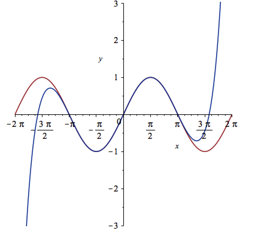
Let’s see how close this is to the sin(x) curve by plotting them both together
plot([sin(x), convert(series(sin(x), x = 0, 10), polynom)], x = -2*Pi .. 2*Pi, y = -3 .. 3);
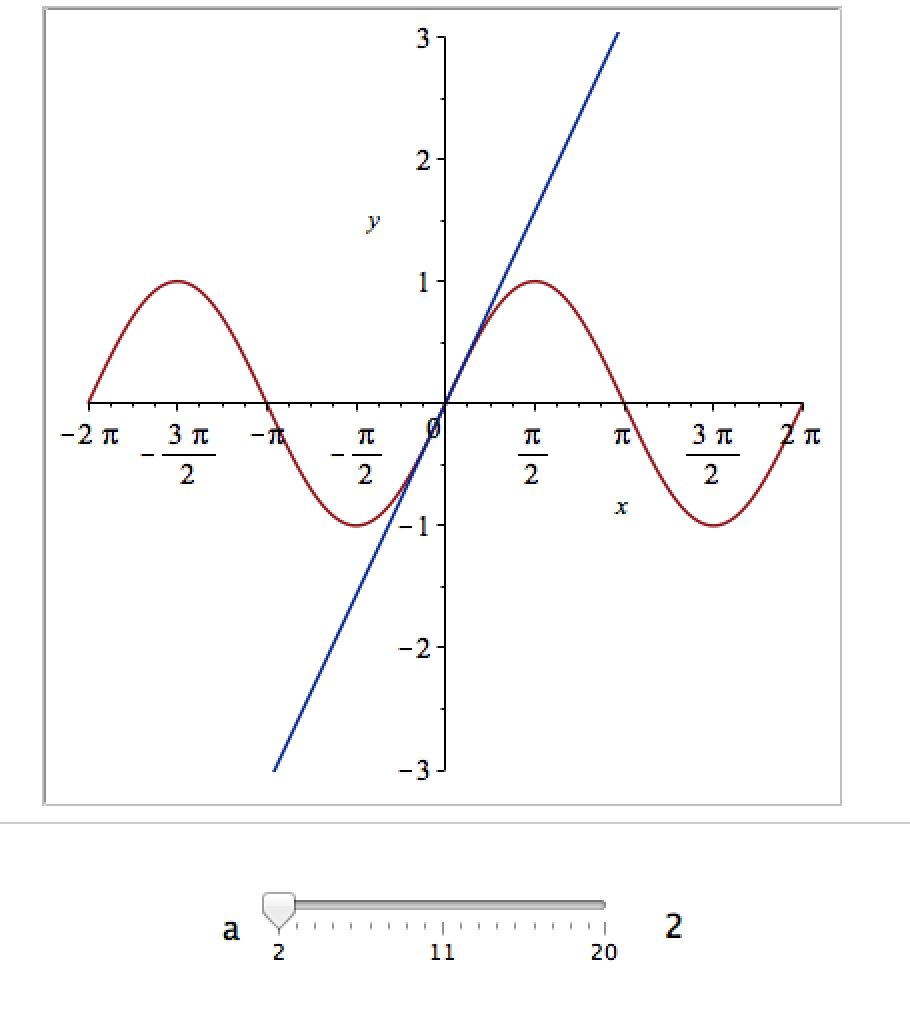
It would be nice if we could see how the approximation varies as we vary the number of terms in the expansion. Change the value 10 to a parameter a, pass the whole thing to the Explore function and we get an interactive widget.
Explore(plot([sin(x), convert(series(sin(x), x = 0, a), polynom)], x = -2*Pi .. 2*Pi, y = -3 .. 3), parameters = [a = 2 .. 20]);
Here’s a screenshot of it:
Adding extra parameters
It would also be nice to vary the point we expand around. Change the value 0 to b and add an extra parameter to Explore to get two sliders instead of one:
Explore(plot([sin(x), convert(series(sin(x), x = b, a), polynom)], x = -2*Pi .. 2*Pi, y = -3 .. 3), parameters = [a = 2 .. 20, b = -2*Pi .. 2*Pi]);
To see what this looks like, open the companion worksheet in Maple.
Adding labels to the sliders
We can change the labels on the sliders as follows
Explore(plot([sin(x), convert(series(sin(x), x = b, a), polynom)], x = -2*Pi .. 2*Pi, y = -3 .. 3), parameters = [[a = 2 .. 20, label = `Number Of Terms`], [b = -2*Pi .. 2*Pi, label = `Expansion location`]]);
To see what this looks like, open the companion worksheet in Maple.
Adding initial values
Finally, let’s set some starting values for each slider
Explore(plot([sin(x), convert(series(sin(x), x = b, a), polynom)], x = -2*Pi .. 2*Pi, y = -3 .. 3), parameters = [[a = 2 .. 20, label = `Number Of Terms`], [b = -2*Pi .. 2*Pi, label = `Expansion location`]], initialvalues = [a = 2, b = 1]);
The resulting interactive widget looks like this:

Not bad for one line of code!
Upload to the Maple Cloud
At The University of Sheffield, we are lucky because all of our staff and students have access to Maple on both university-owned and personally-owned equipment. If your audience isn’t as fortunate, they can access the resulting worksheet on the Maple Cloud.
Update: 2nd July 2015 The code in github has moved on a little since this post was written so I changed the link in the text below to the exact commit that produced the results discussed here.
Imagine that you are a very new MATLAB programmer and you have to create an N x N matrix called A where A(i,j) = i+j
Your first attempt at a solution might look like this
N=2000
% Generate a N-by-N matrix where A(i,j) = i + j;
for ii = 1:N
     for jj = 1:N
         A(ii,jj) = ii + jj;
     end
 end
On my current machine (Macbook Pro bought in early 2015), the above loop takes 2.03 seconds. You might think that this is a long time for something so simple and complain that MATLAB is slow. The person you complain to points out that you should preallocate your array before assigning to it.
N=2000
% Generate a N-by-N matrix where A(i,j) = i + j;
A=zeros(N,N);
for ii = 1:N
     for jj = 1:N
         A(ii,jj) = ii + jj;
     end
 end
This now takes 0.049 seconds on my machine – a speed up of over 41 times! MATLAB suddenly doesn’t seem so slow after all.
Word gets around about your problem, however, and seasoned MATLAB-ers see that nested loop, make a funny face twitch and start muttering ‘vectorise, vectorise, vectorise’. Emails soon pile in with vectorised solutions
% Method 1: MESHGRID.
[X, Y] = meshgrid(1:N, 1:N);
A = X + Y;
This takes 0.025 seconds on my machine — a healthy speed-up on the loop-with-preallocation solution. You have to understand the meshgrid command, however, in order to understand what’s going on here. It’s still clear (to me at least) what its doing but not as clear as the nice,obvious double loop. Call me old fashioned but I like loops…I understand them.
% Method 2: Matrix multiplication.
A = (1:N).' * ones(1, N) + ones(N, 1) * (1:N);
This one is MUCH harder to read but you don’t worry about it too much because at 0.032 seconds it’s slower than meshgrid.
% Method 3: REPMAT.
A = repmat(1:N, N, 1) + repmat((1:N).', 1, N);
This one appears to be interesting! At 0.009 seconds, it’s the fastest so far – by a healthy amount!
% Method 4: CUMSUM.
A = cumsum(ones(N)) + cumsum(ones(N), 2);
Coming in at 0.052 seconds, this cumsum solution is slower than the preallocated loop.
% Method 5: BSXFUN.
A = bsxfun(@plus, 1:N, (1:N).');
Ahhh, bsxfun or ‘The Widow-maker function’ as I sometimes refer to it. Responsible for some of the fastest and most unreadable vectorised MATLAB code I’ve ever written. In this case, it brings execution time down to 0.0045 seconds.
Whenever I see something that can be vectorised with a repmat, I try to figure out if I can rewrite it as a bsxfun. The result is usually horrible to look at so I tend to keep the original loop commented out above it as an explanation! This particular example isn’t too bad but bsxfun can quickly get hairy.
Conclusion
Loops in MATLAB aren’t anywhere near as bad as they used to be thanks to advances in JIT compilation but it can often pay, speed-wise, to switch to vectorisation. The price you often pay for this speed-up is that vectorised code can become very difficult to read.
If you’d like the code I ran to get the timings above, it’s on github (link refers to the exact commit used for this post) . Here’s the output from the run I referred to in this post.
Original loop time is 2.025441
Preallocate and loop is 0.048643
Meshgrid time is 0.025277
Matmul time is 0.032069
Repmat time is 0.009030
Cumsum time is 0.051966
bsxfun time is 0.004527
- MATLAB Version: 2015a
- Early 2015 Macbook Pro with 16Gb RAM
- CPU: 2.8Ghz quad core i7 Haswell
This post is based on a demonstration given by Mathwork’s Ken Deeley during a recent session at The University of Sheffield.