
Archive for January, 2010
There are two carnivals in the mathematics blogging world: The Carnival of Maths (CoM) and Math Teachers at Play (MTAP), which are basically two different facets of the same thing — but exactly what are they?
At the most basic level, a maths carnival is just a set of links to recent blog articles about mathematics, but that’s selling the whole idea short somewhat. I’ve always liked to think that the two carnivals are the shop-front of the mathematics blogging world — a reason for us all to get together and celebrate everything that we are proud of in our little corner of the web. Other people compare a blog carnival to a magazine’s table of contents, which can direct you to a wide variety of articles. The articles are written by different people, but they are all tied together by the theme/focus/area-of-interest that defines the magazine.
The best way of demonstrating what the carnivals are all about is to show you some examples, so here are the two most recent editions (I’ll try to keep this updated):
- Carnival of Mathematics #77 – Jost a mon
- Math Teachers at Play #37 – Math Insider
Let’s look at how the carnivals work in more detail.
Say you have just written a recent mathematical blog post which you are rather proud of. Obviously you’d like as many people as possible to read your article, so you choose one of the two carnivals and submit it using one of the two forms below:
- Carnival of Mathematics submission form (Any kind of maths at any level)
- Math teachers at play submission form (Any kind of maths from preK-12 — which is pretty much all mathematics taught to 19 year olds and below)
The carnivial host will receive your submission and, if they think it is suitable, will include it in their carnival. You can then sit back and watch the extra traffic roll in.
Here are some frequently asked questions about both carnivals.
When are the carnivals published?
The Carnival of Maths usually gets published on the first Friday of the month and Math Teachers at Play gets published on the third Friday.
I would like to host a carnival at my blog. What should I do?
Go to the relevant carnival home page and click on ‘Future Hosts’. This will show you who is scheduled to host for the next few months. Find an empty slot that suits you, contact me for the CoM or Denise for MTAP, and we’ll take it from there.
Who does the admin for the Carnivals?
At the moment, I am doing the admin for the Carnival of Math, and Denise of Let’s Play Math is looking after Math Teachers at Play. So, if you have any questions, then we are your first port of call.
I’ve found a cool maths article that someone else has written. Can I submit it to the carnivals?
Yes, but in an ideal world it will be a recent post and should have never been submitted to one of the carnivals before. The best way to be sure of this, if the post is not your own, is to send in only something published since the last edition of the carnival.
Can I submit an article to both carnivals?
We’d rather you didn’t — at least, not the *same* article. We don’t want to bore the audience.
Who decides what gets included in a carnival and what doesn’t.
The carnival hosts. The carnival is just a guest on the host’s blog, and so what each host writes is entirely up to him or her. In general, most carnival hosts will include almost everything that is submitted to them and a bit more besides. However, if they choose NOT to link to something, then so be it.
The blog carnival server has been known to lose submissions on occasion. I have not heard of trouble with the maths carnivals, but the (much larger) Carnival of Education used to have problems quite often. If you are sure that your article met the carnival guidelines, but the host did not include it, then perhaps it simply got lost. Feel free to resubmit your post for the next edition.
Do I have to be a math teacher to submit an article to Math Teachers at Play?
No. As long as the mathematics is below college-level, then you are good to go
Will the Carnival of Math take articles on basic math?
Yes — everything from kindergaten to cutting edge research is fair game for the Carnival of Math. Basic mathematics can be submitted to either carnival, but advanced maths should generally be submitted only to the Carnival of Math.
Do you accept articles from subjects such as computer science or physics?
As long as there is a reasonable amount of maths content, then yes.
Is there anything else I need to do, besides submitting my article?
No, there is nothing else you have to do. When the carnival is published, however, you may want to post a link to it on your blog. The carnival host will appreciate your support, and your readers will enjoy a chance to browse what other math bloggers have written.
Does the carnival have a twitter feed?
Yes, @Carnivalofmath
![]()
Ever since PTC bought Mathcad from its original developers, Mathsoft, back in 2006 the future for the product has been uncertain. The first PTC-led release of the software, Mathcad 14, followed a few months later to mixed reviews and it’s been very quiet ever since. The only sign of life over the last couple of years has been a few minor bug-fix releases which, to be perfectly frank, is rather insignificant compared to the competition.
All of this led me to write an article back in June 2009 called ‘Is Mathcad Dying?’ which garnered quite a lot of feedback from both the Mathcad user community and from PTC themselves. The reaction from the user community ranged from people calling me some colourful names through to those who agreed with much of what I said and everything in between. It quickly became apparent that there was a large user community who were fervently hoping that PTC would do something special with Mathcad rather than let it wither and die. These users feel that Mathcad brings something unique to the technical software landscape; something that isn’t provided by the likes of Mathematica, MATLAB and Maple and they didn’t want it to go away.
In the meantime, some of the people at PTC got in touch with me to tell me that Mathcad is far from dying. I learned that not only was a new release of Mathcad on the cards (Mathcad 15) but that they were also working on what was essentially a complete reboot of the system called Mathcad Prime. They had also performed an internal company restructure which included the creation of a business unit specifically for Mathcad; this, I was told, would allow them to do much more with Mathcad than had been done before. It all sounded very exciting and I was looking forward to a host of public updates but then it all went very quiet again.
Until now!
One of my contacts at PTC sent me a tweet last night to say that I might be interested in a blog post over at mathcad.wordpress.com and he was right. Finally, everything that I had been told in confidence has been made official and more besides. Mathcad 15 will be released later this year. The date for Mathcad Prime is a little more vague but 2011 seems like a distinct possibility and there will be a virtual conference in mid-March where PTC will tell us more about its Mathcad strategy (I’ve already signed up).
I have to confess that I have never been a fan of Mathcad, preferring to use MATLAB, Mathematica and Maple, but I have been deeply impressed by the loyalty shown by some of its long-term users. Some of these users have been kind enough to take the time to show me why they believe that Mathcad deserves such allegiance and I now realise that some of my earlier comments on the product were not as well thought out as they should have been. So, I hope that these new developments by PTC not only repays this loyalty but also produces a product that I would want to use myself.
Update (1st July 2010): Mathcad 15 has been released now (over 3 years since the last version if I recall correctly) and the list of new features appears to be rather underwhelming at first glance. I’ll write more when I get my copy (assuming that there is more to write about). I guess PTC are putting all of their resources into Mathcad Prime right now.
Ever since version 6 of Mathematica was released (way back in 2007) I have received dozens of queries from users at my University saying something along the lines of ‘Plotting no longer works in Mathematica’ or ‘If I wrap my plot in a Do loop then I get no output. The user usually goes on to say that it worked perfectly well in pre-v6 versions of Mathematica, is clearly a bug and could I please file a bug report with Wolfram Research?
It’s not a bug….it’s a feature!
If you have googled your way here and just want a fast solution to your problem then here goes. I assume that you have code that looks like this
Do[
 Plot[Cos[n x], {x, -Pi, Pi}]
 , {n, 1, 3}
 ]
and you were expecting to get a set of nice plots (in this case 3) – one plot for each iteration of your loop. Instead, Mathematica 6 or above is giving you nothing…nada…zip! There are several ways you can ‘fix’ this and I am going to show you two. Option 1 is to wrap your Plot Command with Print
Do[
 Print[Plot[Cos[n x], {x, -Pi, Pi}]]
 , {n, 1, 3}
 ]
Option 2 is to use Table instead of Do
Table[
 Plot[Cos[n x], {x, -Pi, Pi}]
 , {n, 1, 3}
 ]
I am imaging that the average googler has now disappeared having got what they came for but some of you are possibly wondering why the above two ‘fixes’ work. Here’s my attempt at an explanation.
Old versions of Mathematica (v5.2 and below) treated graphics very differently to the way that Mathematica works today. The output of a command such as Plot[] used to contain two parts – the first was a Graphics object which looked a bit like the following in the notebook front end
– Graphics –
This was the OutputForm of the actual symbolic result of the Plot[] command. The second part – the actual visualization of the plot – was effectively just a side effect that happened to be what us humans actually wanted.
In version 6 and above, the OutputForm of a Graphics object is its visualisation which makes a lot more sense then just – Graphics –. The practical upshot of this is that there is now no need for a ‘side effect’ since the visualization of the plot IS the output. If you are confused then this bit is explained much more eloquently in an old Wolfram Blog post.
That’s the first part of the story regarding plots in loops. The second piece of the puzzle is to know that when you wrap a Mathematica expression in a Do loop then you suppress its output but you don’t suppress any side effects. In version 5.2 the plot is a side effect and so it gets displayed on each iteration of the loop. In version 6 and above, the plot is the output and so gets suppressed unless you explicitly ask for it to be displayed using Print[].
Does this help clear things up? Comments welcomed.
The Numerical Algorithms Group (NAG) is 40 years old this year and they have begun their celebrations by starting a company blog. In their first blog post, one of the numerical library developers has asked the world a question:
“How useful would routines that provide particular solutions to the Painleve equations be to our customer base and to the research community in particular?”
I’ll confess that, until 10 minutes ago, I had never heard of the Painlevé equations but there are articles on Wikipedia and Mathworld to get you started if you are in the same boat as me.
If, on the other hand, you know all about them and can venture an opinion then head over to NAG’s new blog and say hi.
I am a big fan of the NAG’s products and you can see some of my posts about them at the following links:
- PyNAG – My Python wrappers for the NAG C-library
- A faster version of MATLAB’s interp1 function – using the NAG Toolbox for MATLAB
- NAG: The ultimate MATLAB toolbox – A mini-review of NAG’s MATLAB toolbox
- Calling the NAG Library from Excel
Did you make any New Year’s resolutions this year? If you did then who will they help? Just you? Your family? Your students? The whole world? If I am being honest then I have to say that most of the new-year’s resolutions I have made over the years tend to focus on myself because at my very core I am a bit selfish. So, my resolutions tend to be things like “I want to get fitter”, “I’ll not stay late at work so much” or “I want to learn more Python programming.”
If I keep these resolutions then I’m going to be fitter, more knowledgeable and have a better work-life balance. So far so selfish!
Over the last few days though I have made a rather different sort of new-years resolution. Yes, I admit that it’s a bit late but why limit change to an essentially arbitrary date? My new new year’s resolution is to give a little back to the community that has given me so much – the community of organisations and individuals who provide me with software – either for free or for such a trivial amount of money that it may as well be free.
Now I am not a rich man so I can’t give away great wads of cash and although I am a programmer I have neither the time nor the knowledge to provide significant amounts of code to any particualr project. So what can I do?
Donations
Well, although I am not minted, I can easily afford the occasional small donation or two so I will start making them. It’s already begun with my Sage bounty hunt and will continue with other projects over the year. Another small donation I made recently was to buy the ‘Premium’ version of Aldiko – a great ebook reader for Android smartphones. Aldiko is a free piece of software, has been downloaded by tens of thousands of users and is used by me on an almost daily basis. I noticed that they had a ‘Premium’ version available for $1.99 but it turns out that it is identical to the free version. The $1.99 simply represents a donation to the developers and it’s a donation I made without hesitation. Doing the right thing for less than two dollars – getting the warm fuzzies has never been easier!
Bug reports and feedback
Thanks to my job and to running Walking Randomly I get to see how researchers, teachers, students and average joes use mathematical software quite a lot. I get told about bugs, about feature wish lists, about gripes with licensing, performance issues…the list goes on and on. The best way to get bugs fixed is to report them – first tell the developers and, if the bug is interesting/severe enough, tell the world. I do this plenty with commercial software but I am going to make the effort more with free software from now on. Feedback is part of the lifeblood of free software and developers need both the good and the bad.
Did you try out Octave, Maxima, Sage or Smath Studio and it didn’t work out? Why didn’t it? What did these packages have missing that forced you to turn to alternatives? Try to be specific; saying ‘I tried it and it sucks’ is a rubbish piece of feedback because it’s just an opinion and gives the developers nothing to do. Saying something like ‘I tried to calculate XYZ and it gave the following incorrect result whereas it should have given ABC’ is MUCH more productive.
Tutorials, examples and documentation
One comment I have heard over and over again from people who have tried free mathematical software and then turned their back on it is that the ‘documentation isn’t good enough’. These people want more tutorials, more examples, more explanations and just more and better documentation. Do you like writing? Do you like fiddling with math software? I do and so I intend on giving as many examples and tutorials as I can. I also have a (moderately) successful blog so I can provide a publishing outlet for people who want to write such things but don’t want to start a blog of their own. This has already begun too with Greg Astley’s tutorial on how to plot direction fields for ODE’s in maxima. Contact me if you are interested in doing this yourself and we’ll discuss it.
Talk
I like to talk. Many people who know me personally would probably go so far as to say I talk too much but I can use this to help towards my new resolution too. I’m going to give short talks, demonstrations and seminars on free mathematical software to interested people over the coming year via various fora. Maybe you could too?
So, in summary, I plan to do the following to give back to free software over the next decade and I invite you to do the same.
- Give small, direct donations to some of my favourite open source and free software projects
- Set up bounty hunts for particular features I want in various packages
- Buy donation versions of Android software whenever possible
- Publish as many examples of using software such as Sage, octave and maxima as I can
- Help write tutorials and documentation
- Give talks to help spread the word
I’ll admit that none of this will change the world but it will possibly help a few more people than “I resolve to get myself fitter.”
I recently received a notification about the 2010 International Mathematica Symposium (IMS) which is due to take place in Beijing, China from July 16th this year. The IMS is not run by Wolfram Research (although I think that Wolfram is a sponsor) but is run by Mathematica enthusiasts for Mathematica enthusiasts. I was lucky enough to be able to attend both the 2008 IMS in Maastricht and the 2006 IMS in Avignon where I had a fantastic time, learned lots of stuff and met loads of people who just love Mathematica and mathematics.
I have to say that I have never been to a conference quite like the IMS before; the attendees were simply fizzing with enthusiasm and the range of talks and activities were wonderful. In Avignon, I learned how to use Manipulate even before Mathematica 6 was released. In Maastrict I was among the first to see some of the new features in Mathematica 7 and have seen Mathematica applied to subject areas as diverse as cancer research, high school math teaching, puzzle solving, quantum mechanics, electronics, radio astronomy and finance. I’ve been taught Mathematica tricks from some of the very people who wrote the thing and have swapped programming methods and scripts with users of all levels.
The knowledge base of those attending the IMS ranges from people who eat, breathe and sleep Mathematica through to people who have only just started using it and everything in between. I’ve met (and now consider among my friends) a statistics expert from Australia, a genetic algorithms expert from Canada and a college instructor from Finland among many others. I’ve celebrated Mathematica’s 20th birthday in some underground caves, had my head read and also got a couple of very nice T-shirts which I love but my wife refuses to be seen with (she doesn’t like my MATLAB T-shirts either)!
There is usually a sprinkling of Wolfram employees among the attendees which gives you the chance to get the inside track on what is going on within Wolfram Research. If you have a problem understanding something in Mathematica or there is a bug that winds you up then who better to talk to? The IMS has also given me the chance to meet the authors of some of the most well known Mathematica books over the years which was fantastic. Discussing a fun math problem with people like this and then watching them cook up a cool looking demonstration in minutes will surely get your imagination fired up.
Unfortunately, due to a distinct lack of funds, I probably won’t be at the IMS in Beijing but if you are into Mathematica and can make it there then I highly suggest you go. You won’t regret it and I’d appreciate it if someone could send me the T-Shirt ;)
This is the first post on Walking Randomly that isn’t written by me! I’ve been thinking about having guest writers on here for quite some time and when I first saw the tutorial below (written by Manchester University undergraduate, Gregory Astley) I knew that the time had finally come. Greg is a student in Professor Bill Lionheart’s course entitled Asymptotic Expansions and Perturbation Methods where Mathematica is the software of choice.
Now, students at Manchester can use Mathematica on thousands of machines all over campus but we do not offer it for use on their personal machines. So, when Greg decided to write up his lecture notes in Latex he needed to come up with an alternative way of producing all of the plots and he used the free, open source computer algebra system – Maxima. I was very impressed with the quality of the plots that he produced and so I asked him if he would mind writing up a tutorial and he did so in fine style. So, over to Greg….
This is a short tutorial on how to get up and running with the “plotdf” function for plotting direction fields/trajectories for 1st order autonomous ODEs in Maxima. My immediate disclaimer is that I am by no means an expert user!!! Furthermore, I apologise to those who have some experience with this program but I think the best way to proceed is to assume no prior knowledge of using this program or computer algebra systems in general. Experienced users (surely more so than me) may feel free to skip the ‘boring’ parts.
Firstly, to those who may not know, this is a *free* (in both the “costs no money”, and “it’s open source” senses of the word) computer algebra system that is available to download on Windows, Mac OS, and Linux platforms from http://maxima.sourceforge.net and it is well documented.
There are a number of different themes or GUIs that you can use with the program but I’ll assume we’re working with the somewhat basic “Xmaxima” shell.
Install and open up the program as you would do with any other and you will be greeted by the following screen.
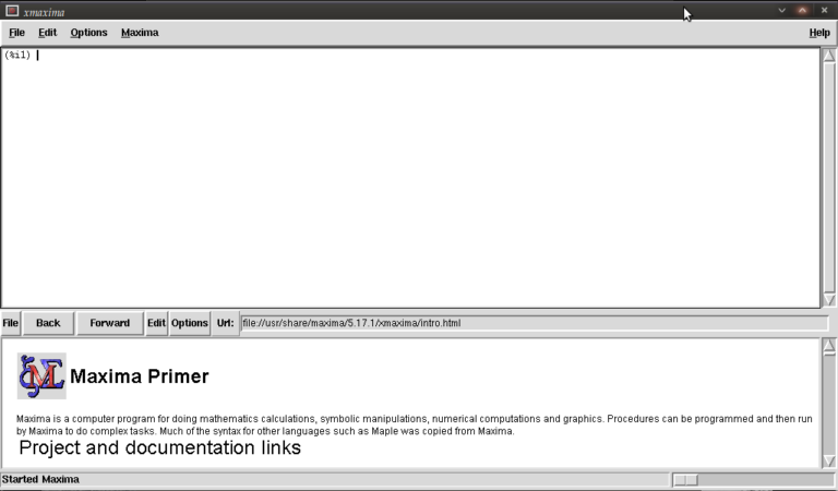
You are meant to type in the top most window next to (%i1) (input 1)
We first have to load the plotdf package (it isn’t loaded by default) so type:
load("plotdf");
and then press return (don’t forget the semi-colon or else nothing will happen (apart from a new line!)). it should respond with something similar to:
(%i1)  load("plotdf");
(%o1)  /usr/share/maxima/5.17.1/share/dynamics/plotdf.lisp
(%i2)
We will now race ahead and do our first plot. Keeping things simple for now we’ll do a phase plane plot for dx/dt = y, dy/dt = x, type:
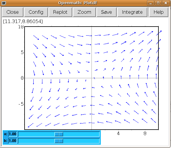
plotdf([y,x]);
you should see something like this:
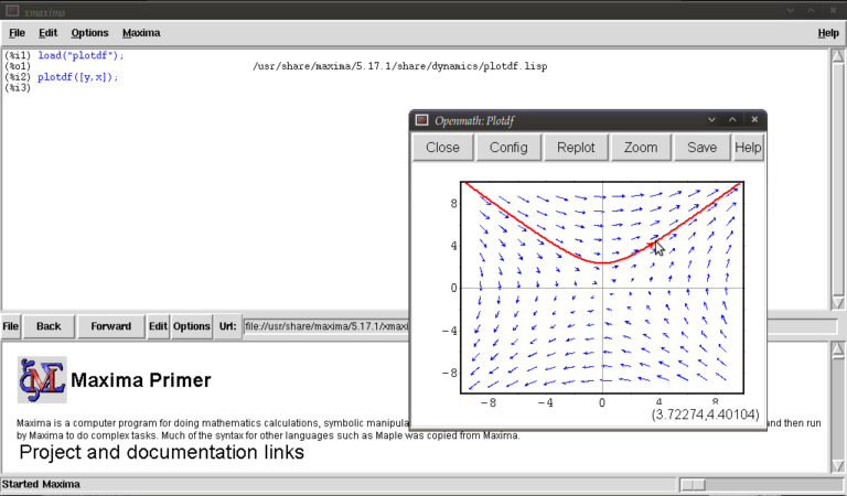
This is the Openmath plot window, (there are other plotting environments like Gnuplot but this function works only with Openmath) Notice that my pointer is directly below a red trajectory. These plots are interactive, you can draw other trajectories by clicking elsewhere. Try this. Hit the “replot” button and it will redraw the direction field with just your last trajectory.
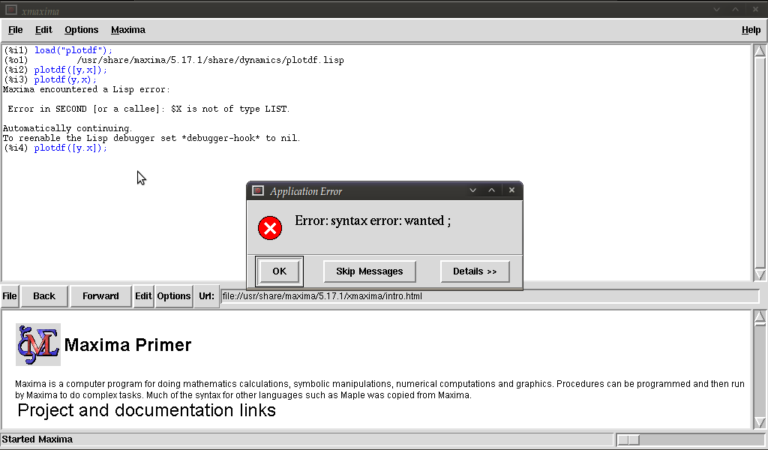
Before exploring any other options I want to purposely type some bad input and show how to fix things when it throws an error or gets stuck. Type
plotdf(y,x);
it should return
(%i3) plotdf(x,y);
Maxima encountered a Lisp error:

Error in SECOND [or a callee]: $Y is not of type LIST.

Automatically continuing.
To enable the Lisp debugger set *debugger-hook* to nil.
(%i4)
We forgot to put our functions for dx/dt,dy/dt in a list (square brackets). This is a reasonably safe error in that it tells us it isn’t happy and lets us continue.
Now type
plotdf([x.y]);
you should see something similar to
The problem this time was that we typed a dot instead of a comma (easily done), but worryingly when we close this message box and the blank plot the program will not process any commands. This can be fixed by clicking on the following in the xmaxima menu
file >> interrupt
where after telling you it encountered an error it should allow you to continue. One more; type
plotdf([2y,x]);
It should return with
  (%i5) plotdf([2y,x]);
  Incorrect syntax: Y is not an infix operator
  plotdf([2y,
           ^
  (%i5)
This time we forgot to put a binary operation such as * or + between 2 and y. If you come up with any other errors and the interrupt command is of no use you can still partially salvage things via
file >> restart
but you will, in this case, have to load plotdf again. (mercifully you can go to the line where you first typed it and press return (as with other commands you might have done))
I will now demonstrate some more “contrived” plots (for absolutely no purpose other than to shamelessly give a (very) small gallery of standard functions/operations etc… for the novice user) there is no need to type the last four unless you want to see what happens by changing constants/parameters, they’re the same plot :)
  plotdf([2*y-%e^(3/2)+cos((%pi/2)*x),log(abs(x))-%i^2*y]);
  plotdf([integrate(2*y,y)/y,diff((1/2)*x^2,x)]);
  plotdf([(3/%pi)*acos(1/2)*y,(2/sqrt(%pi))*x*integrate(exp(-x^2),x,0,inf)]);
  plotdf([floor(1.43)*y,ceiling(.35)*x]);
  plotdf([imagpart(x+%i*y),(sum(x^n,n,0,2)-sum(x^j,j,0,1))/x]);
I could go on…notice that the constants pi, e, and i are preceded by “%”. This tells maxima that they are known constants as opposed to symbols you happened to call “pi”, “e”, and “i”. Also, noting that the default range for x and y is (-10,10) in both cases; feel free to replot the first of those five without wrapping x inside “abs()” (inside the logarithm that is). remember file >> interrupt afterwards!
Now I will introduce you to some more of the parameters you can plug into “plotdf(…)”. close any plot windows and type
plotdf([x,y],[x,1,5],[y,-5,5]);
You should notice that x now ranges from 1 to 5, whilst y ranges from -5 to 5. There is nothing special about these numbers, we could have chosen any *real* numbers we liked. You can also use different symbols for your variables instead of x or y. Try
plotdf([v,u],[u,v]);
Note that I’ve declared u and v as variables in the second list. I will now purposely do something wrong again. Assign the value 5 to x by typing
x:5;
then type
plotdf([y,x]);
This time maxima won’t throw an error because syntactically you haven’t done anything wrong, you merely told it to do
plotdf([y,5]);
as opposed to what you really wanted which is
plotdf([y,x]);
Surprisingly to me (discovered as I’m writing this), changing the names of your variables like we did above won’t save you since it seems to treat new symbols as merely placeholders for it’s favourite symbols x and y. To get round this type
kill(x);
and this will put x back to what it originally was (the symbol x as opposed to 5).
You don’t actually have to provide expressions for dx/dt and dy/dt, you might instead know dy/dx and you can generate phaseplots by typing say
plotdf([x/y]);
In this case we didn’t actually need the square brackets because we are providing only one parameter: dy/dx (x will be set to t by maxima giving dx/dt = 1, and dy/dt = dy/dx = x/y)
A number of parameters can be changed from within the openmath window. Type
plotdf([y,x],[trajectory_at,-1,-2],[direction,forward]);
and then go into config. The screen you get should look something like this:
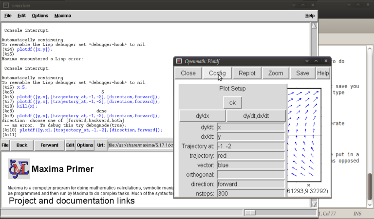
from here you can change the expressions for dx/dt, dy/dt, dy/dx, you can change colours and directions of trajectories (choices of forward, backward, both), change colours for direction arrows and orthogonal curves, starting points for trajectories (the two numbers separated by a space here, not a comma), time increments for t, number of steps used to create an integral curve. You can also look at an integral plots for x(t) and y(t) corresponding to the starting point given (or clicked) by hitting the “plot vs t” button. You can also zoom in or out by hitting the “zoom” button and clicking (or shift+clicking to unzoom), doing something else like hitting the config button will allow you to quit being in zoom mode click for trajectories again. (there might be a better way of doing this btw) You can also save these plots as eps files (you can then tweak these in other vector graphics based programs like Inkscape (free) or Adobe Illustrator etc..)
Interactive sliders
There are many permutations of things you can do (and you will surely find some of these by having a play) but my particular favourite is the option to use sliders allowing you to vary a parameter interactively and seeing what happens to the trajectories without constant replotting. ie:
plotdf([a*y,b*x],[sliders,"a=-1:3,b=-1:3"]);
Hopefully, this has been enough to get people started, and for what it’s worth, the help file (though using xmaxima, you’ll find this in the web-browser version) for this topic has a pretty good gallery of different plots and other parameters I didn’t mention.
just to throw in one last thing in the spirit of experimentation, is the following set of commands:
A:matrix([0,1],[1,0]);
B:matrix([x],[y]);
plotdf([A[1].B,A[2].B);
which is another way of doing the same old
plotdf([y,x]);
where here I’ve made a 2×2 matrix A, a 2×1 matrix B, with A[1], A[2] denoting rows 1 and 2 of A respectively and matrix multiplied the rows of A by B (using A[1].B, A[2].B) to serve as inputs for dx/dt and dy/dt
Tutorial written by Gregory Astley, Mathematics Undergraduate at The University of Manchester.
I’m really late doing this article and it has already been done very well by MathNotations and 360. There’s also a nice game involving the number 2010 over at Let’s play math. They didn’t mention this fact though
2010 = 1+2-(3-4-5)*6*7*8-9
Which I think is nice. Do you have any more interesting facts about the number 2010?
Today is a big day! Not only is it the first day of the new year but it’s also the first day of a new decade! In addition to all of that it is also time for the 61st Carnival of Mathematics and this one has shaped up to be a great one thanks to the growing army of carnival contributors out there. So, put off joining the gym for one more day; Sit back, relax and enjoy this feast of pulchritudinous mathematics.
First off, as per long standing carnival tradition, let’s look at some interesting properties of the number 61. Well, it’s prime for a start but so are a lot of numbers so maybe that isn’t so interesting. However, 61 is the smallest multidigit prime p such that the sum of digits of p^p is a square (pop-quiz – what is the next one?). While on the subject of primes, 61 is the smallest prime who’s digit reversal is square! It also turns out that the 61st Fibonacci number (2504730781961) is the smallest Fibonacci number which contains all the digits from 0 to 9. (Thanks to Number Gossip for these by the way).
So 61 is a lot more interesting than you thought huh? If it had a name then it would be Keith and he would be Australian.

Puzzles, games and problems.
Let’s kick things off with a few puzzles. Sam Shah has submitted a problem for you to try which was originally created by his sister (A physics teacher) in A stubborn equilateral triangle.
If you are in the market for some online math games and lessons then head over to TutorFi.com and see what Meaghan Montrose has found for you.
Jonathan has a very interesting puzzle over at his blog, jd2718, called Who Am I (Teacher Edition) which should keep you thinking while you recover from the new year festivities.
Finally, Erich Friedman has prepared a set of holiday puzzles for 2009 for you all to try.
Explorations, discussions and messing about with maths
Pi is irrational right? Have you ever seen the proof? If not then you need to check out Brent Yorgey’s three part series on the irrationality of Pi over at The Math Less Travelled. Part 3 of this series forms Brent’s submission to today’s carnival.
Pat Ballew has had his math class working on some maximization problems recently and his article Exploring an Isoperimetric Theme discusses a discovery about a “rule of thumb” for some maximization problems. In a later post he wonders if there is a relation between the shape of a polygon and the maxium length of the diagonals (for a fixed perimeter).
Something that has kept potamologists awake over the years is the geometry of meandering rivers. If you’ve ever wondered about the same thing then head over to Division by Zero to see what Dave Richeson has to say on the subject.
Terry Tao has been getting into the holiday season with a ‘more frivolous post than usual’ in A demonstration of the non-commutativity of the English language while Qiaochu Yuan of Annoying Precision gets more serious and considers the combinatorics of words in The cyclotomic identity and Lyndon words.

Matters of a statistical nature
John D. Cook has been contemplating questions involving rare diseases and counterfeit coins over at The Endeavour.
Over at An Ergodic Walk the author has been discussing a statistical problem of how to estimate a probability distribution from samples when you don’t know e.g. how many possible values there are. An example application is estimating the number of different butterfly species from a sample containing many unique species.
I don’t know about you but I like to have a game of cards with my mates from time to time (Poker is our usual game of choice and I am fantastically bad at it). Every now and then a small ‘discussion’ breaks out concerning how shuffled the deck of cards is which is usually solved by somone reshuffling them ‘properly’. But how many suffles are necessary to randomize a deck of cards? Mathematically, card-shuffling can be viewed as a random walk on a finite group and, thus, it can be modeled by a Markov chain. Rod Carvalho has the details.
Techno Techno Techno….the technological side of mathematics
Sage is one of the best free mathematical software packages you can get at the moment and the project is led by William Stein, an associate professor at The University of Washington. In his post Mathematical Software and Me he discusses his past experiences with mathematical software and recounts the series of events that led him to start the development of Sage. If you are interested in Sage and can program in Python and Javascript then you may want to consider my Sage Bounty Hunt.
Wolfram Alpha has been a big hit among mathematics bloggers this year and, since it was launched back in May, Wolfram Research have added a lot of new features to it. For a list of some of the more recent features check out the latest post from the Wolfram Alpha Blog – New Features in Wolfram|Alpha: Year-End Update.
Visualisation of volume data is getting easier every day thanks to products such as MATLAB and Patrick Kalita recently gave an internal talk to Mathworks engineers explaining how to do it. This talk was recorded and turned into a series of 9 blog posts by Doug Hull over at Doug’s MATLAB Video Tutorials and the final part was posted early in December.
Teaching, learning and testing
Explaining mathematics can be hard and there are many different ways of teaching it. In How We Teach, Joel Feinstein shares some of his methodologies and includes a screencast of a talk of his entitled “Using a tablet PC and screencasts when teaching mathematics.”
Every year, many hundreds of mathematics graduate students take language exams where they translate some technical writing in French,German or Russian into English. These translations are then graded and thrown away which seems like a waste of effort when you think about it. David Speyer wonders if there is a more useful way to administer language exams in his post Let’s make language exams useful.
Finally, Eric Mazur has posted a ‘video confession’ on YouTube saying “I thought I was a good teacher until I discovered my students were just memorizing information rather than learning to understand the material. Who was to blame?”
Happy new Year – Math Carnival Style!
Now that it is officially 2010 you will be in need of a new calendar which is where Ron Doerfler of Dead Reckonings comes in. He has created a great looking calendar called The Age of Graphical Computing and has made it all available for free. Just download, print and away you go. I have to confess that I am too lazy to build them myself and so only wish that he could make them available for sale somehow. What about it Ron?
So, that’s it for this edition of the carnival – I hope you enjoyed it. The next one will be published on February 4th and I am still looking for someone to host it. So, if you have blog about mathematics and would like a traffic boost then drop me a line and we’ll discuss it.