Walking Randomly

Last month I (along with half of the blogging world it seems) reported on a new project from Wolfram Research called Wolfram Alpha.  At the time I didn’t know much about it but since then much more information has been available.

Rather than write more about it myself, I will simply refer you to the information I have seen.  First of all, the video below is a recording of a talk given by Stephen Wolfram about the project a couple of days ago.  Click here if you prefer to watch this directly on YouTube.

Secondly, a new blog has started up called (predictably enough) The Wolfram Alpha blog.   The first article is called The Quest for Computable Knowledge: A Longer View.

Many people are comparing Wolfram Alpha to Google which is completely wrong as far as I can tell.  It’s a bit like comparing a table of logarithms with a computer algebra system (CAS) that can calculate any logarithm you like, in any base along with the ability to plot a graph of any function that contains a logarithm.  The CAS can also differentiate, integrate, and simplify equations containing logarithms and so on.  The table of logarithms contains pre-computed data that you can search whereas the CAS can do computations based on your ‘searches’ on the fly.

Let’s take an example from the talk that Stephen gave.  Say you enter

6000C

(I assume this is what he entered, the video wasn’t so hot on showing the overhead projector connected to his laptop.  I’d give good money to get some slides right now)

Wolfram Alpha tries to tell you something useful about this input drawing from the data-sets that it has access to.  It also COMPUTES potentially useful things from these data sets.  It’s the computation part that makes it fundamentally different from google (NOTE: I said different from, not better than or a competitor to – the distinction is important in my opinion).

Wolfram Alpha will say something like ‘assuming that C is a unit and assuming that unit is Celsius then I can tell you the following about 6000C’  It will then go on to tell you various conversion factors (such as, I guess, what it would be in degrees Fahrenheit or Kelvin).  It might plot the black body spectrum at 6000 degrees C and show what colour a black-body object at that temperature would be.

All of these results will have been computed from scratch based upon various mathematical formulae and models that Wolfram Alpha has access to.  Google, on the other hand, would only show the black body spectrum at 6000C if someone had calculated it in advance and put it up on a webpage.

Of course Wolfram Alpha knows a lot more than just temperatures.  It knows about weather statistics, economic data, the human genome, properties of materials, symbolic integrals (and how to do them by hand) and loads more.

Looks like an exciting project!  I wonder how Wolfram will make money out if it (or even if it intends to)?

OK, so with today’s release of Maple version 13, this blog post is a little late but I started so I’ll finish! My original install of Maple was 12.01 on Ubuntu Linux and a little while ago an update was released to take this to version 12.02.

Installation

In theory I should be able to install this automagically by clicking on Tools->Check for Updates inside Maple. However, when I did this I was told that ‘no updates were currently available‘ so I had to download the update manually from here. I was very pleased to note that this update was offered free of charge to all Maple 12 users. This is exactly as it should be and other software vendors should take note here – users don’t like paying for bug-fix updates! Well done to Maplesoft for doing it right. Once I had downloaded the 12.02 update installer, the installation itself was pretty straightforward. The following incantations did the trick for me

chmod +x ./Maple1202Linux32Upgrade.bin
sudo ./Maple1202Linux32Upgrade.bin

A graphical installer fired up and all I had to do was click Next a couple of times and point it to my Maple 12.01 installation. A few seconds later it was all over.  It’s a shame that the automatic checker didn’t work but all in all this was a very painless experience!

Now since this update only increments the version number by 0.01 you shouldn’t be expecting any marvellous new features.  What you should be expecting is some tidying up and bug fixing and that is exactly what you get.  Maplesoft’s own description of the bug-fixes weren’t detailed enough for my tastes and so I appealed to my informants at Maplesoft for something more explicit.

Happily, they delivered and most of what follows is from them.  Thanks Maplesoft :)

Since 12.02 was released along with the launch of MapleSim, many of the updates were geared towards symbolic manipulation and simplification, which is always beneficial for any advanced computations, but very important for MapleSim. As such, the best examples to illustrate the updates are in MapleSim, and are not easily shown with a Maple example alone. More specifically though, there were other enhancements and fixes that were added to Maple 12.02 to help improve it, which are not tied directly to MapleSim:

Updates to dsolve

There were two significant issues present in Maple 12.01 and earlier that are not present in Maple 12.02. One of these deals with a certain class of singularities that are transparent to explicit rk-pair based numerical solvers.

As the simplest example in this class, the differential system:

dsys := {diff(x(t),t)=x(t)/(1-t),x(0)=1};

having the exact solution:

dsolve(dsys);

has a singularity at t=1, and exactly ‘0’ error according to explicit rk-pair error estimation.

This, and other related singularities (such as jump discontinuities) are now detected to provide an accurate numerical solution. Compare this output from 12.01

dsn := dsolve(dsys, numeric);

 dsn := proc(x_rkf45)  ...  end proc

dsn(0.999);

[t = .999, x(t) = -48.3295522342053872]

dsn(1.001);

[t = 1.001, x(t) = -48.4646844943701609]

with the improved output from 12.02

dsn := dsolve(dsys, numeric);

 dsn := proc(x_rkf45)  ...  end proc

dsn(0.999);

 [t = 0.999, x(t) = 1000.00023834227034]

dsn(1.001);

Error, (in dsn) cannot evaluate the solution further right of
.99999999, probably a singularity

The second fix deals with error control on index-1 (non-differential) variables in the problem. This can be seen if you take a trivial problem coupled with a non-trivial index-1 variable. For example: In Maple 12.01:

dsys := {diff(x(t),t)=1, y(t)=sin(t), x(0)=0}:
 dsn := dsolve(dsys, numeric):
 dsn(Pi);

[t = 3.14159265358979, x(t) = 3.14159265358978956,
     y(t) = -0.00206731654642018647]

dsn(2*Pi);

[t = 6.28318530717958, x(t) = 6.28318530717958357,
     y(t) = -0.0623375491269087187]

The ‘y’ value should have been zero. In Maple 12.02:

dsys := {diff(x(t),t)=1, y(t)=sin(t), x(0)=0}:
 dsn := dsolve(dsys, numeric):
 dsn(Pi);

[t = 3.14159265358979, x(t) = 3.14159265358978956,
     y(t) = -0.117631599366556372 10^-6  ]

dsn(2*Pi);

[t = 6.28318530717958, x(t) = 6.28318530717958090,
     y(t) = -0.130170125786817359 10^-6  ]

which is zero within the default error tolerances.

Plot Annotations bug fix

In 12.01, some plot annotations were not appearing as expected. When a text box was entered on a 2D plot, the text would not appear until focus was taken away from the text box itself. For example, if you were to create a plot of sin(x) plot(sin(x)) and then click on the plot, select drawing from the toolbar and then select ‘T’ to enter a text field, you could begin typing, but would not receive visual feedback of what you entered until you clicked outside of the textbox. Obviously, this was a bug, and it was fixed in 12.02.

Improvements to embedded components

Prior to 12.02, some installations of Linux displayed some issues with redrawing of various embedded components, which slowed down scrolling in a Maple document. In 12.02, Maplesoft added a few fixes to the way that they handle embedded components, especially for 32-bit systems, which took care of this issue for most Linux installations. Also, since they were in the area, they took the opportunity to tweak response times for embedded components when creating them and executing the code that dictates their behavior in a document. This is not *very* noticeable when you have just a few components in a document, but it becomes very visible with Maplesoft’s interactive ebooks and with user applications that rely on a large number of components in a single application.

Excel Link improvements

In Maple, there is a built-in link to Microsoft Excel, so that you can perform Maple computations within an Excel spreadsheet. Maplesoft started supporting Excel 2007 in Maple 12, but with a service pack release to Windows released shortly thereafter and some security enhancements added to Maple, the link did not perform as expected in 12.01. Certain values were being interpreted incorrectly, as such, Maplesoft felt that they needed to address these inconsistencies as soon as possible. So for 12.02, they fixed the link for Excel 2007 to ensure that values were faithfully being passed from Microsoft Excel to Maple, in order to maintain the connection and computation accuracy.

No sooner had I installed the Maple 12.02 update and wrote a blog post on it (to be published soon) than Maple 13 is released! I haven’t had chance to take a detailed look at everything that’s new (It was only released a few hours ago) but MapleSoft have prepared a series of great short videos that show off the new functionality.

Some highlights from my point of view are (the following links are to MapleSoft and will open a new browser window containing a video)

• The Student Numerical Analysis Package
• Fly through animations of 3d graphs
• Multithreaded Task programming (or how to use all of the cores of your dual/quad core processor)

I’ll try and write more as soon as I get any extra information – right after the blog post concerning new functionality in Maple 12.02!  So much stuff to write about, so little time :(

The latest version of the powerful free, open-source maths package, SAGE, was released last week.  Version 3.4.1 brings us a lot of new functionality compared to 3.4 and the SAGE team have prepared a detailed document showing us why the upgrade is worthwhile.

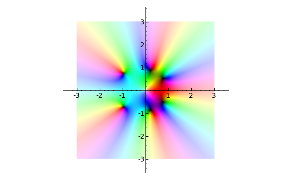
For example, the new complex_plot function looks fantastic.  From the documentation:

The function complex_plot() takes a complex function f(z) of one variable and plots output of the function over the specified xrange and yrange. The magnitude of the output is indicated by the brightness (with zero being black and infinity being white), while the argument is represented by the hue with red being positive real and increasing through orange, yellow, etc. as the argument increases.

sage: f(z) = z^5 + z - 1 + 1/z
sage: complex_plot(f, (-3, 3), (-3, 3))

Sage aims to become a ‘viable free open source alternative to Magma, Maple, Mathematica and Matlab’ and I think it is well on the way.  I become a little more impressed with it with every release and I am a hardcore Mathematica and MATLAB fan.

One major problem with it (IMHO at least) is that there is no native windows version which prevents a lot of casual users from trying it out.  Although you can get it working on Windows, it is far from ideal because you have to run a virtual machine image using VMWare player.  The hard-core techno geeks among you might well be thinking ‘So what?  Sounds easy enough.’ but it’s an extra level of complexity that casual users simply do not want to have to concern themselves with.  Of course there is also the issue of performance – emulating an entire machine to run a single application is hardly a good use of compute resources.

There is a good reason why SAGE doesn’t have a proper Windows version yet – it’s based upon a lot of component parts that don’t have Windows versions and someone has to port each and every one of them.  It’s going to be a lot of work but I think it will be worth it.

When the SAGE development team release a native Windows version of their software then I have no doubt that it will make a significant impact on the mathematical software scene – especially in education.  There will be nothing preventing every school and university in the world from having access to a world-class computer algebra system.

In an ideal world everyone would be running Linux but we don’t live in an ideal world so a Windows version of SAGE would be a step in the right direction.

Update: It turns out that a Windows port is being developed and something should be ready soon – http://windows.sagemath.org/ Thanks to mvngu in the comments section for pointing this out. I should have done my research better!

Someone I know recently gave me a heads up about a cool looking calculator for the iPhone called Pi Cubed from Sunset Lake Software.  I haven’t been able to test this because I don’t have the hardware but it looks like quite a nice way to use the iPhone as a calculator -the user interface is completely different to any other calculator I have seen.

Features include

• 34 digits of decimal precision
• A database of over 150 built-in equations from Finance, basic maths, physics, fluid mechanics etc.
• All variables in the built-in equations are annotated so you don’t need to remember what each term stands for.
• Email equations from the iphone in either plain text or Latex formats.
• Built in reference manual.
• Many built in scientific functions such as trig and inverse trig functions, logarithms to any real base, roots to any real power (square root, cube root etc), the error function and factorials.

Check out the video below for more details (streamed from the developer’s website)

I’ve just discovered a blog bost where the author was installing Octave on a Mac.  Looks hard!

I compare it with Ubuntu’s installation method for Octave along with the symbolic package:

sudo apt-get install octave octave-symbolic

and wonder what is going wrong for it on Macs.  Insights anyone?

This is part 5 of a series of articles devoted to demonstrating how to call the Numerical Algorithms Group (NAG) C library from Python.  Click here for the index to this series.

The Optimisation chapter of the NAG C library is one of the most popular chapters in my experience.  It is also one of the most complicated from a programming point of view but if you have been working through this series from the beginning then you already know all of the Python techniques you need.  From this point on it’s just a matter of increased complexity.

As always, however, I like to build the complexity up slowly so let’s take a look at possibly the simplest NAG optimisation routine – e04abc.  This routine minimizes a function of one variable, using function values only.  In other words – you don’t need to provide it with derivative information which simplifies the programming at the cost of performance.

The example Python code I am going to give will solve a very simple local optimisation problem – The minimisation of the function sin(x)/x in the range [3.5,5.0] or, put another way, what are the x and y values of the centre of the red dot in the picture below.

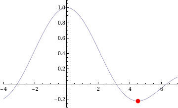
The NAG/Python code to do this is given below (or you can download it here).

#!/usr/bin/env python
#Example 4 using NAG C library and ctypes - e04abc
#Mike Croucher - April 2008
#Concepts : Communication callback functions that use the C prototype void funct(double, double *,Nag_comm *)

from ctypes import *
from math import *
libnag = cdll.LoadLibrary("/opt/NAG/cllux08dgl/lib/libnagc_nag.so.8")
e04abc = libnag.e04abc
e04abc.restype=None

class Nag_Comm(Structure):
	_fields_ = [("flag", c_int),
                ("first", c_int),
 		("last", c_int),
		("nf",c_int),
		("it_prt",c_int),
		("it_maj_prt",c_int),
		("sol_sqp_prt",c_int),
		("sol_prt",c_int),
		("rootnode_sol_prt",c_int),
		("node_prt",c_int),
		("rootnode_prt",c_int),
		("g_prt",c_int),
		("new_lm",c_int),
		("needf",c_int),
		("p",c_void_p),
		("iuser",POINTER(c_int) ),
		("user",POINTER(c_double) ),
		("nag_w",POINTER(c_double) ),
		("nag_iw",POINTER(c_int) ),
		("nag_p",c_void_p),
		("nag_print_w",POINTER(c_double) ),
		("nag_print_iw",POINTER(c_int) ),
		("nrealloc",c_int)
		]

#define python objective function
def py_obj_func(x,ans,comm):
  ans[0] = sin(x) / x
  return

#create the type for the c callback function
C_FUNC = CFUNCTYPE(None,c_double,POINTER(c_double),POINTER(Nag_Comm))

#now create the c callback function
c_func = C_FUNC(py_obj_func)

#Set up the problem parameters
comm = Nag_Comm()
#e1 and e2 control the solution accuracy.  Setting them to 0 chooses the default values.
#See the documentation for e04abc for more details
e1 = c_double(0.0)
e2 = c_double(0.0)
#a and b define our starting interval
a = c_double(3.5)
b = c_double(5.0)
#xt will contain the x value of the minimum
xt=c_double(0.0)
#f will contain the function value at the minimum
f=c_double(0.0)
#max_fun is the maximum number of function evaluations we will allow
max_fun=c_int(100)
#Yet again I cheat for fail parameter.
fail=c_long(0)

e04abc(c_func,e1,e2,byref(a),byref(b),max_fun,byref(xt),byref(f),byref(comm),fail)

print "The minimum is in the interval  [%s,%s]" %(a.value,b.value)
print "The estimated result = %s" % xt.value
print "The function value at the minimum is %s " % f.value
print "%s evaluations were required" % comm.nf

If you run this code then you should get the following output

The minimum is in the interval  [4.4934093959,4.49340951173]
The estimated result = 4.49340945381
The function value at the minimum is -0.217233628211
10 evaluations were required

IFAIL oddness

My original version of this code used the trick of setting the NAG IFAIL parameter to c_int(0) to save me from worrying about the NagError structure (this is first explained in part 1) but when this example was tested it didn’t work on 64bit machines although it worked just fine on 32bit machines.  Changing it to c_long(0) (as I have done in this example)  made it work on both 32 and 64bit machines.

What I find odd is that in all my previous examples, c_int(0) worked just fine on both architectures.  Eventually I will cover how to use the IFAIL parameter ‘properly’ but for now it is sufficient to be aware of this issue.

Scary Structures

Although this is the longest piece of code we have seen so far in this series, it contains no new Python/ctypes techniques at all. The only major difficulty I faced when writing it for the first time was making sure that I got the specification of the Nag_Comm structure correct by carefully working though the C specification of it in the nag_types.h file (included with the NAG C library installation) and transposing it to Python.

One of the biggest hurdles you will face when working with the NAG C library and Python is getting these structure definitions correct and some of them are truly HUGE. If you can get away with it then you are advised to copy and paste someone else’s definitions rather than create your own from scratch. In a later part of this series I will be releasing a Python module called PyNAG which will predefine some of the more common structures for you.

Callback functions with Communication

The objective function (that is, the function we want to minimise) is implemented as a callback function but it is a bit more complicated than the one we saw in part 3.  This NAG routine expects the C prototype of your objective function to look like this:

void funct(double xc, double *fc, Nag_Comm *comm)

• xc is an input argument and is the point at which the value of f(x) is required.
• fc is an output argument and is the value of the function f at the current point x.  Note that it is a pointer to double.
• Is a pointer to a structure of type Nag_Comm.  Your function may or may not use this directly but the NAG routine almost certainly will.  It is through this structure that the NAG routine can communicate various things to and from your function as and when is necessary.

so our C-types function prototype looks like this

C_FUNC = CFUNCTYPE(None,c_double,POINTER(c_double),POINTER(Nag_Comm))

whereas the python function itself is

#define python objective function
def py_obj_func(x,ans,comm):
  ans[0] = sin(x) / x
  return

Note that we need to do

ans[0] = sin(x) / x

rather than simply

ans = sin(x) / x

since ans is a pointer to double rather than just a double.

In this particular example I have only used the simplest feature provided by the Nag_Comm structure and that is to ask it how many times the objective function was called.

print "%s evaluations were required" % comm.nf

That’s it for this part of the series. Next time I’ll be looking at a more advanced optimisation routine. Feel free to post any comments, questions or suggestions.

When I bought my Dell XPS M1330 it had Ubuntu Hardy Heron (8.04) installed and I quickly upgraded to Intrepid Ibex (8.10) using the update manager with only minor problems. Well, after today’s release of version 9.04 of Ubuntu, otherwise known as Jaunty Jackalope, I decided to jump on the bandwagaon and upgrade yet again.

It never ceases to amaze me how easy it is to go from one version of Ubuntu to another.  I just typed the following in the terminal and followed the instructions

sudo update-manager -d

A couple of hours or so later and I had a shiny new operating system up and running.  Lot’s of people have written about the new stuff in this latest version of Ubuntu so I won’t repeat any of that but what I will do is report on how the upgrade affected (or otherwise) some of my favourite mathematical programs.

• Mathematica 7.0 seems to have been unaffected and works just fine.
• MATLAB 2009a seems to be just fine too.
• Maple 12.01 is working perfectly.

How very dull!  Nothing to fix at all with these three.

Youtube sound problems

For some reason there is no sound on Youtube videos.  The following fix is touted by some but it didn’t work for me as I already had the package installed

sudo apt-get install flashplugin-nonfree-extrasound

So far I haven’t managed to find a fix for this issue but will update this page if that changes.

Sound is too quiet (FIXED)

The sound output on the M1330 has always been on the quiet side but as of this update it is so quiet that I can barely hear a thing (and before you ask – yes I have checked that the volume is set to maximum.  Hopefully I’ll find a fix for this too.

Update:OK so it turns out that I didn’t have ALL the volume sliders turned up to maximum.  The path to success lay in installing and running gnome-alsamixer.

sudo apt-get install gnome-alsamixer
gnome-alsamixer

and then ensure that all of the sliders are turned up to maximum.  MUCH better!

I’ll update this page as I find out more info.

Like many math bloggers, I was starting to worry that the Carnival of Maths had died a death after John hosted the excellent 50th edition.  However, that’s not the case, it was just resting.  The carnival is alive and well and it looks like it will be hosted over at Squarecirclez tomorrow.  If you are a blogger and have recently written something mathematical then head over to the Carnival submission form and submit it.

You know you want to!

Imagine that you were the Captain of a sailing ship a few hundred years ago and, in order to protect yourself from pirates, you had a few cannons.  Cannons need cannonballs and it is well known that the best way to stack cannon balls is to arrange them as a square pyamid as in the image below.

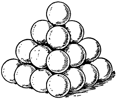
So, in this example you have 16 balls in the bottom layer, 9 balls in the next layer, then 4 and, finally, one at the top giving a total of 16+9+4+1 = 30 balls and we say that 30 is the 4th square pyramidal number.  The first few such numbers are

• 1
• 5 (4+1)
• 14 (9+4+1)
• 30 (16+9+4+1)
• 55 (25+16+9+4+1)

Now, there is a well known problem called the Cannonball problem (Spolier alert: This link contains the solution) which asks ‘What is the smallest square number that is also square pyramidal number?’ but the traditional cannonball problem has been stated and solved by many people and so it isn’t my problem of the week.

My problem is as follows ‘Consider a square pyramidal pile of identical cannonballs of radius r such that the bottom layer contains 16 cannonballs (such as the pile in the diagram above). Find the volume (in terms of r) of the pyramid that envelops and contains the whole pile‘

As always, there are no prizes I’m afraid (but if you are a company who would like to sponsor prizes for future POTWs then let me know).  I imagine that the solution to this will require a diagram so it might be best to put your solution on a pdf file, web page or some other visual media rather than using the comments section.  Finding my email adress is yet another (easy) puzzle to solve.

Have fun.