
Archive for the ‘mathematica’ Category
I learned about entropy as part of my undergraduate Physics education but it turns out that the concept of entropy turns up in many fields including linguistics, themodynamics, information theory, chemistry and artificial intelligence.
As part of Sheffield’s Open Data Science Initiative, computer scientist, Neil Lawrence, has teamed up with linguist, Dagmar Divjak, to organise a cross-faculty discussion meeting on the subject of entropy.
For more details on the day’s events, and to register, see http://opendsi.cc/ed2016/program

I wasted a little time producing the above logo for the event using Mathematica.
Here’s the source code:-
(*consider column one pixel at a time. Invert the pixel if a random number is below some threshold*)
flipbit[col_, prob_] := Module[{result, temp, x},
  result = col;
  Do[
   If[RandomReal[] <=  prob,
    If[result[[x]] == 1, result[[x]] = 0, result[[x]] = 1];
    ]
   , {x, 1, Length[col]}
   ];

  Return[result]
  ]

text = "Entropy";
image = Rasterize[Text[Style[text, White, Italic, 190]],
   Background -> Black];
imageData = ImageData[Binarize[image]];
const = 1/Dimensions[imageData][[2]]*0.42;
(*Apply flipbit to all columns. Increase probability of flipping as you move along the x-axis*)
logo =
  Transpose[
   MapIndexed[flipbit[#1, const*#2[[1]]] &, Transpose[imageData]]];
Image[logo]
Finally, I found this quote about entropy that I quite like:
You should call it entropy, for two reasons. In the first place your uncertainty function has been used in statistical mechanics under that name, so it already has a name. In the second place, and more important, no one really knows what entropy really is, so in a debate you will always have the advantage.
John von Neumann to Claude Shannon a name for his new uncertainty function. Source: Wikiquotes
I’ve been working at The University of Manchester for almost a decade and will be leaving in just less than 3 weeks time! A huge part of my job was to support a major subset of Manchester’s site licensed application software portfolio so naturally I’ve made use of a lot of it over the years. As of February 20th, I will no longer be entitled to use any of it!
This article is the first in a series where I’ll look at some of the software that’s become important to me and what my options are on leaving Manchester.
Here, I consider Mathematica – a computer algebra system and technical computing environment that I’m very fond of. I’ve been a Mathematica user for over 15 years and yet, suddenly, I find myself license-less! So much code, so much time invested! What to do?
Options for all use cases
- Before leaving University, contact the administrator of your site license. It could be that you are entitled to a discount on buying one of the various licenses on offer.
- Use the CDF Player – With this free tool, You’ll be able to look at and interact (at least partially) with Mathematica notebooks.
- Re-write all code to use something else. Which language to use is open to massive debate but the closest open source systems to Mathematica’s notebook-like interface are Jupyter (previously IPython) and Sage. The languages are, of course, rather different though!
Hobbyist use
General mucking around!
- Buy the home edition – The home edition of Mathematica can be used for non-professional and non-academic purposes and, at the time of writing, costs £195 as a one-off cost or £95 per year.
- Use Mathematica online: Home – Same rules as the home edition above but it’s a cloud-based, online version. Currently costs £95 per year.
- Buy a Raspberry Pi – The Raspberry Pi comes with a free version of Mathematica! This means that you can buy an entire computer AND a copy of Mathematica for less than the standard home-use license. I had a play with Mathematica on the Raspberry Pi just over a year ago and it was very nice. Now that the faster, more powerful Raspberry Pi 2 has been released this option is even more compelling!
Academic use
If you want to use Mathematica in an academic environment that doesn’t have a site license, you’ll need to purchase an individual academic license. At the time of writing, that will cost £860 + VAT.
Professional use
There are various grades of professional license and the cost varies according to how many compute kernels you need or Wolfram Alpha API calls you want to make. Current prices start at £2,035 +VAT
RLink is Mathematica’s interface to the R language – a feature that has been extremely popular since its debut in Mathematica version 9. It’s a great package but has one or two issues. For example, RLink makes use of a built in version of R which is currently stuck at the rather old version 2.14. Official support for the use of external versions of R and adding third-party libraries varies by operating system and version of Mathematica. Windows support is great — OS X support, not so much.
Expert Mathematica user Szabolcs Horvát has written the definitive guide on how to get RLink up and running with the latest version of R on all three major operating systems, building on earlier work by Leonid Shifrin and members of the Mathematica Stack Exchange community. Thanks to this work, we can now enjoy any version of R we like with Mathematica!
Introduction
Mathematica 10 was released yesterday amid the usual marketing storm we’ve come to expect for a new product release from Wolfram Research. Some of the highlights of this marketing information include
- Mathematica 10 blog post by Stephen Wolfram
- What’s new in 10? From Wolfram Research
- Alphabetical list of new functions
Without a doubt, there is a lot of great new functionality in this release and I’ve been fortunate enough to have access to some pre-releases for a while now. There is no chance that I can compete with the in-depth treatments given by Wolfram Research of the 700+ new functions in Mathematica 10 so I won’t try. Instead, I’ll hop around some of the new features, settling on those that take my fancy.
Multiple Undo
I’ve been a Mathematica user since version 4 of the product which was released way back in 1999. For the intervening 15 years, one aspect of Mathematica that always frustrated me was the fact that the undo feature could only undo the most recent action. I, along with many other users, repeatedly asked for multiple undo to be implemented but were bitterly disappointed for release after release.
Few things have united Mathematica users more than the need for multiple undo:
- A website with petition calling for multiple undo
- A Facebook page calling for multiple undo
- A very popular Mathematica StackExchange question about multiple undo
Finally, with version 10, our hopes and dreams have been answered and multiple undo is finally here. To be perfectly honest, THIS is the biggest reason to upgrade to version 10. Everything else is just tasty gravy.
Key new areas of functionality
Most of the things considered in this article are whimsical and only scratch the surface of what’s new in Mathematica 10. I support Mathematica (and several other products) at the University of Manchester in the UK and so I tend to be interested in things that my users are interested in. Here’s a brief list of new functionality areas that I’ll be shouting about
- Machine Learning I know several people who are seriously into machine learning but few of them are Mathematica users. I’d love to know what they make of the things on offer here.
- New image processing functions The Image Processing Toolbox is one of the most popular MATLAB toolboxes on my site. I wonder if this will help turn MATLAB-heads. I also know people in a visualisation group who may be interested in the new 3D functions on offer.
- Nonlinear control theoryVarious people in our electrical engineering department are looking at alternatives to MATLAB for control theory. Maple/Maplesim and Scilab/Xcos are the key contenders. SystemModeler is too expensive for us to consider but the amount of control functionality built into Mathematica is useful.
Entities – a new data type for things that Mathematica knows stuff about
One of the new functions I’m excited about is GeoGraphics that pulls down map data from Wolfram’s servers and displays them in the notebook. Obviously, I did not read the manual and so my first attempt at getting a map of the United Kingdom was
GeoGraphics["United Kingdom"]
What I got was a map of my home town, Sheffield, surrounded by a red cell border indicating an error message
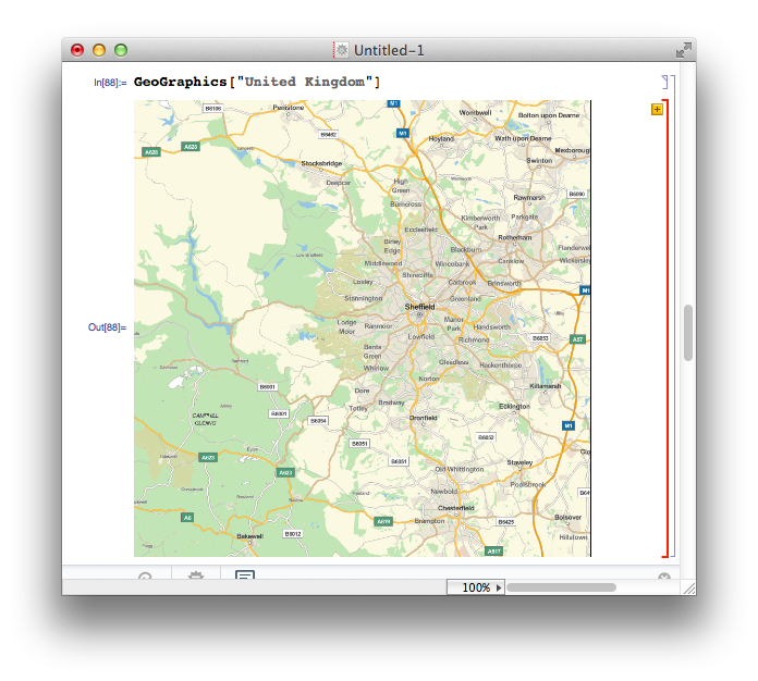
The error message is “United Kingdom is not a Graphics primitive or directive.” The practical upshot of this is that GeoGraphics is not built to take strings as arguments. Fair enough, but why the map of Sheffield? Well, if you call GeoGraphics[] on its own, the default action is to return a map centred on the GeoLocation found by considering your current IP address and it seems that it also does this if you send something bizarre to GeoGraphics. In all honesty, I’d have preferred no map and a simple error message.
In order to get what I want, I have to pass an Entity that represents the UK to the GeoGraphics function. Entities are a new data type in Mathematica 10 and, as far as I can tell, they formally represent ‘things’ that Mathematica knows about. There are several ways to create entities but here I use the new Interpreter function
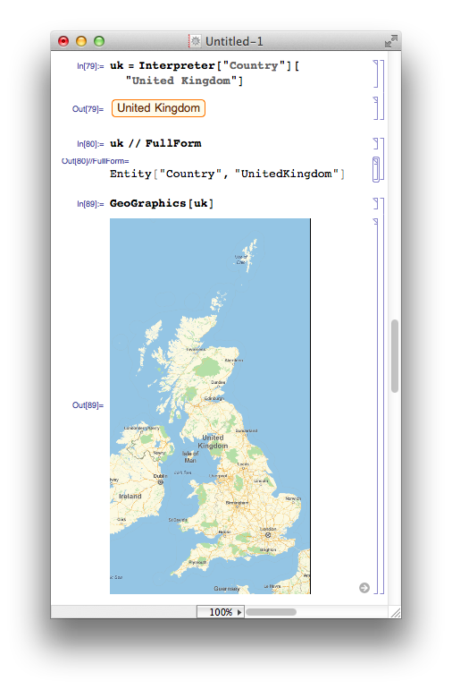
From the above, you can see that Entities have a special new StandardForm but their InputForm looks straightforward enough. One thing to bear in mind here is that all of the above functions require a live internet connection in order to work. For example, on thinking that I had gotten the hang of the Entity syntax, I switched off my internet connection and did
mycity = Entity["City", "Manchester"]

During evaluation of In[92]:= URLFetch::invhttp: Couldn't resolve host name. >>

During evaluation of In[92]:= WolframAlpha::conopen: Using WolframAlpha requires internet connectivity. Please check your network connection. You may need to configure your firewall program or set a proxy in the Internet Connectivity tab of the Preferences dialog. >>

Out[92]= Entity["City", "Manchester"]
So, you need an internet connection even to create entities at this most fundamental level. Perhaps it’s for validation? Turning the internet connection back on and re-running the above command removes the error message but the thing that’s returned isn’t in the new StandardForm:
![]()
If I attempt to display a map using the mycity variable, I get the map of Sheffield that I currently associate with something having gone wrong (If I’d tried this out at work,in Manchester, on the other hand, I would think it had worked perfectly!). So, there is something very wrong with the entity I am using here – It doesn’t look right and it doesn’t work right – clearly that connection to WolframAlpha during its creation was not to do with validation (or if it was, it hasn’t helped). I turn back to the Interpreter function:
In[102]:= mycity2 = Interpreter["City"]["Manchester"] // InputForm

Out[102]//InputForm:= Entity["City", {"Manchester", "Manchester", "UnitedKingdom"}]
So, clearly my guess at how a City entity should look was completely incorrect. For now, I think I’m going to avoid creating Entities directly and rely on the various helper functions such as Interpreter.
What are the limitations of knowledge based computation in Mathematica?
All of the computable data resides in the Wolfram Knowledgebase which is a new name for the data store used by Wolfram Alpha, Mathematica and many other Wolfram products. In his recent blog post, Stephen Wolfram says that they’ll soon release the Wolfram Discovery Platform which will allow large scale access to the Knowledgebase and indicated that ‘basic versions of Mathematica 10 are just set up for small-scale data access.’ I have no idea what this means and what limitations are in place and can’t find anything in the documentation.
Until I understand what limitations there might be, I find myself unwilling to use these data-centric functions for anything important.
IntervalSlider – a new control for Manipulate
I’ll never forget the first time I saw a Mathematica Manipulate – it was at the 2006 International Mathematica Symposium in Avignon when version 6 was still in beta. A Wolfram employee created a fully functional, interactive graphical user interface with just a few lines of code in about 2 minutes –I’d never seen anything like it and was seriously excited about the possibilities it represented.
8 years and 4 Mathematica versions later and we can see just how amazing this interactive functionality turned out to be. It forms the basis of the Wolfram Demonstrations project which currently has 9677 interactive demonstrations covering dozens of fields in engineering, mathematics and science.
Not long after Mathematica introduced Manipulate, the sage team introduced a similar function called interact. The interact function had something that Manipulate did not – an interval slider (see the interaction called ‘Numerical integrals with various rules’ at http://wiki.sagemath.org/interact/calculus for an example of it in use). This control allows the user to specify intervals on a single slider and is very useful in certain circumstances.
As of version 10, Mathematica has a similar control called an IntervalSlider. Here’s some example code of it in use
Manipulate[
 pl1 = Plot[Sin[x], {x, -Pi, Pi}];
 pl2 = Plot[Sin[x], {x, range[[1]], range[[2]]}, Filling -> Axis,
   PlotRange -> {-Pi, Pi}];
 inset = Inset["The Integral is approx " <> ToString[
     NumberForm[
      Integrate[Sin[x], {x, range[[1]], range[[2]]}]
      , {3, 3}, ExponentFunction -> (Null &)]], {2, -0.5}];
 Show[{pl1, pl2}, Epilog -> inset], {{range, {-1.57, 1.57}}, -3.14,
  3.14, ControlType -> IntervalSlider, Appearance -> "Labeled"}]
and here’s the result:

Associations – A new kind of brackets
Mathematica 10 brings a new fundamental data type to the language, associations. As far as I can tell, these are analogous to dictionaries in Python or Julia since they consist of key,value pairs. Since Mathematica has already used every bracket type there is, Wolfram Research have had to invent a new one for associations.
Let’s create an association called scores that links 3 people to their test results
In[1]:= scores = <|"Mike" -> 50.2, "Chris" -> 100.00, "Johnathan" -> 62.3|>

Out[1]= <|"Mike" -> 50.2, "Chris" -> 100., "Johnathan" -> 62.3|>
We can see that the Head of the scores object is Association
In[2]:= Head[scores]

Out[2]= Association
We can pull out a value by supplying a key. For example, let’s see what value is associated with “Mike”
In[3]:= scores["Mike"]

Out[3]= 50.2
All of the usual functions you expect to see for dictionary-type objects are there:-
In[4]:= Keys[scores]

Out[4]= {"Mike", "Chris", "Johnathan"}

In[5]:= Values[scores]

Out[5]= {50.2, 100., 62.3}

In[6]:= (*Show that the key "Bob" does not exist in scores*)
KeyExistsQ[scores, "Bob"]

Out[6]= False
If you ask for a key that does not exist this happens:
In[7]:= scores["Bob"]

Out[7]= Missing["KeyAbsent", "Bob"]
There’s a new function called Counts that takes a list and returns an association which counts the unique elements in the list:
In[8]:= Counts[{q, w, e, r, t, y, u, q, w, e}]

Out[8]= <|q -> 2, w -> 2, e -> 2, r -> 1, t -> 1, y -> 1, u -> 1|>
Let’s use this to find something out something interesting, such as the most used words in the classic text, Moby Dick
In[1]:= (*Import Moby Dick from Project gutenberg*)

MobyDick =
  Import["http://www.gutenberg.org/cache/epub/2701/pg2701.txt"];
(*Split into words*)
words = StringSplit[MobyDick];
(*Convert all words to lowercase*)

words = Map[ToLowerCase[#] &, words];
(*Create an association of words and corresponding word count*)

wordcounts = Counts[words];
(*Sort the association by key value*)

wordcounts = Sort[wordcounts, Greater];
(*Show the top 10*)
wordcounts[[1 ;; 10]]

Out[6]= <|"the" -> 14413, "of" -> 6668, "and" -> 6309, "a" -> 4658,
 "to" -> 4595, "in" -> 4116, "that" -> 2759, "his" -> 2485,
 "it" -> 1776, "with" -> 1750|>
All told, associations are a useful addition to the Mathematica language and I’m happy to see them included. Many existing functions have been updated to handle Associations making them a fundamental part of the language.
- How to make use of Associations? – a question from Mathematica Stack Exchange
s/Mathematica/Wolfram Language/g
I’ve been programming in Mathematica for well over a decade but the language is no longer called ‘Mathematica’, it’s now called ‘The Wolfram Language.’ I’ll not lie to you, this grates a little but I guess I’ll just have to get used to it. Flicking through the documentation, it seems that a global search and replace has happened and almost every occurrence of ‘Mathematica’ has been changed to ‘The Wolfram Language’
This is part of a huge marketing exercise for Wolfram Research and I guess that part of the reason for doing it is to shift the emphasis away from mathematics to general purpose programming. I wonder if this marketing push will increase the popularity of The Wolfram Language as measured by the TIOBE index? Neither ‘Mathematica’ or ‘The Wolfram Language’ is listed in the top 100 and last time I saw more detailed results had it at number 128.
Fractal exploration
One of Mathematica’s competitors, Maple, had a new release recently which saw the inclusion of a set of fractal exploration functions. Although I found this a fun and interesting addition to the product, I did think it rather an odd thing to do. After all, if any software vendor is stuck for functionality to implement, there is a whole host of things to do that rank higher in most user’s list of priorities than a function that plots a standard fractal.
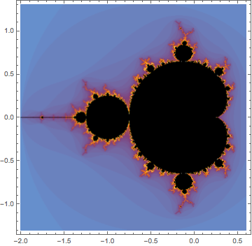
It seems, however, that both Maplesoft and Wolfram Research have seen a market for such functionality. Mathematica 10 comes with a set of functions for exploring the Mandelbrot and Julia sets. The Mandelbrot set alone accounts for at least 5 of Mathematica 10’s 700 new functions:- MandelbrotSetBoettcher, MandelbrotSetDistance, MandelbrotSetIterationCount, MandelbrotSetMemberQ and MandelbrotSetPlot.
MandelbrotSetPlot[]
Barcodes
I found this more fun than is reasonable! Mathematica can generate and recognize bar codes and QR codes in various formats. For example
BarcodeImage["www.walkingrandomly.com", "QR"]

Scanning the result using my mobile phone brings me right back home :)
Unit Testing
A decent unit testing framework is essential to anyone who’s planning to do serious software development. Python has had one for years, MATLAB got one in 2013a and now Mathematica has one. This is good news! I’ve not had chance to look at it in any detail, however. For now, I’ll simply nod in approval and send you to the documentation. Opinions welcomed.
Disappointments in Mathematica 10
There’s a lot to like in Mathematica 10 but there’s also several aspects that disappointed me
No update to RLink
Version 9 of Mathematica included integration with R which excited quite a few people I work with. Sadly, it seems that there has been no work on RLink at all between version 9 and 10. Issues include:
- The version of R bundled with RLink is stuck at 2.14.0 which is almost 3 years old. On Mac and Linux, it is not possible to use your own installation of R so we really are stuck with 2.14. On Windows, it is possible to use your own installation of R but CHECK THAT version 3 issue has been fixed http://mathematica.stackexchange.com/questions/27064/rlink-and-r-v3-0-1
- It is only possible to install extra R packages on Windows. Mac and Linux users are stuck with just base R.
This lack of work on RLink really is a shame since the original release was a very nice piece of work.
If the combination of R and notebook environment is something that interests you, I think that the current best solution is to use the R magics from within the IPython notebook.
No update to CUDA/OpenCL functions
Mathematica introduced OpenCL and CUDA functionality back in version 8 but very little appears to have been done in this area since. In contrast, MATLAB has improved on its CUDA functionality (it has never supported OpenCL) every release since its introduction in 2010b and is now superb!
Accelerating computations using GPUs is a big deal at the University of Manchester (my employer) which has a GPU-club made up of around 250 researchers. Sadly, I’ll have nothing to report at the next meeting as far as Mathematica is concerned.
FinancialData is broken (and this worries me more than you might expect)
I wrote some code a while ago that used the FinancialData function and it suddenly stopped working because of some issue with the underlying data source. In short, this happens:
In[12]:= FinancialData["^FTAS", "Members"]

Out[12]= Missing["NotAvailable"]
This wouldn’t be so bad if it were not for the fact that an example given in Mathematica’s own documentation fails in exactly the same way! The documentation in both version 9 and 10 give this example:
In[1]:= FinancialData["^DJI", "Members"]

Out[1]= {"AA", "AXP", "BA", "BAC", "CAT", "CSCO", "CVX", "DD", "DIS", \
"GE", "HD", "HPQ", "IBM", "INTC", "JNJ", "JPM", "KFT", "KO", "MCD", \
"MMM", "MRK", "MSFT", "PFE", "PG", "T", "TRV", "UTX", "VZ", "WMT", \
"XOM"}
but what you actually get is
In[1]:= FinancialData["^DJI", "Members"]

Out[1]= Missing["NotAvailable"]
For me, the implications of this bug are far more reaching than a few broken examples. Wolfram Research are making a big deal of the fact that Mathematica gives you access to computable data sets, data sets that you can just use in your code and not worry about the details.
Well, I did just as they suggest, and it broke!
Summary
I’ve had a lot of fun playing with Mathematica 10 but that’s all I’ve really done so far – play – something that’s probably obvious from my choice of topics in this article. Even through play, however, I can tell you that this is a very solid new release with some exciting new functionality. Old-time Mathematica users will want to upgrade for multiple-undo alone and people new to the system have an awful lot of toys to play with.
Looking to the future of the system, I feel excited and concerned in equal measure. There is so much new functionality on offer that it’s almost overwhelming and I love the fact that its all integrated into the core system. I’ve always been grateful of the fact that Mathematica hasn’t gone down the route of hiving functionality off into add-on products like MATLAB does with its numerous toolboxes.
My concerns center around the data and Stephen Wolfram’s comment ‘basic versions of Mathematica 10 are just set up for small-scale data access.’ What does this mean? What are the limitations and will this lead to serious users having to purchase add-ons that would effectively be data-toolboxes?
Final
Have you used Mathematica 10 yet? If so, what do you think of it? Any problems? What’s your favorite function?
Mathematica 10 links
- Playing with Mathematica on Raspberry Pi – The Raspberry Pi was the first platform that saw Mathematica version 10…and it’s free!
A recent Google+ post from Mathemania4u caught my attention on the train to work this morning. I just had to code up something that looked like this and so fired up Mathematica and hacked away. The resulting notebook can be downloaded here. It’s not particularly well thought through so could almost certainly be improved on in many ways.
The end result was a Manipulate which you’ll be able to play with below, provided you have a compatible Operating System and Web browser. The code for the Manipulate is
Manipulate[
 Graphics[Map[dotCirc,
   circArray[circrad, theta, pointsize, extent, step, phase,
    showcirc]]]
 , {{showcirc, True, "Show Circles"}, {True, False}}
 , {{theta, 0, "Dot Angle"}, 0, 2 Pi, Pi/10, Appearance -> "Labeled"}
 , {{pointsize, 0.018, "Dot Size"}, 0, 1, Appearance -> "Labeled"}
 , {{phase, 2, "Phase Diff"}, 0, 2 Pi, Appearance -> "Labeled"}
 , {{step, 0.25, "Circle Separation"}, 0, 1, Appearance -> "Labeled"}
 , {{extent, 2, "Plot Extent"}, 1, 5, Appearance -> "Labeled"}
 , {{circrad, 0.15, "Circle Radius"}, 0.01, 1, Appearance -> "Labeled"}
 , Initialization :>
  {
   dotCirc[{x_, y_, r_, theta_, pointsize_, showcirc_}] := If[showcirc,
     {Circle[{x, y}, r], PointSize[pointsize],
      Point[{x + r Cos[theta], y + r Sin[theta]}]}
     ,
     {PointSize[pointsize],
      Point[{x + r Cos[theta], y + r Sin[theta]}]}]
   ,
   circArray[r_, theta_, pointsize_, extent_, step_, phase_,
     showcirc_] := Module[{},
     Partition[
      Flatten[Table[{x, y, r, theta + x*phase + y*phase, pointsize,
         showcirc}, {x, -extent, extent, step}, {y, -extent, extent,
         step}]], 6]
     ]}]
If you can use the Manipulate below, I suggest clicking on the + icon to the right of the ‘Dot Angle’ field to expose the player controls and then press the play button to kick off the animation.
I also produced a video – The code used to produce this is in the notebook.
)
I found these links a while ago and forgot to post them here. Some interesting insights.
A question I get asked a lot is ‘How can I do nonlinear least squares curve fitting in X?’ where X might be MATLAB, Mathematica or a whole host of alternatives. Since this is such a common query, I thought I’d write up how to do it for a very simple problem in several systems that I’m interested in
This is the Mathematica version. For other versions,see the list below
- Simple nonlinear least squares curve fitting in Maple
- Simple nonlinear least squares curve fitting in Julia
- Simple nonlinear least squares curve fitting in MATLAB
- Simple nonlinear least squares curve fitting in Python
- Simple nonlinear least squares curve fitting in R
The problem
You have the following 10 data points
xdata = -2,-1.64,-1.33,-0.7,0,0.45,1.2,1.64,2.32,2.9
ydata = 0.699369,0.700462,0.695354,1.03905,1.97389,2.41143,1.91091,0.919576,-0.730975,-1.42001
and you’d like to fit the function

using nonlinear least squares. You’re starting guesses for the parameters are p1=1 and P2=0.2
For now, we are primarily interested in the following results:
- The fit parameters
- Sum of squared residuals
Future updates of these posts will show how to get other results such as confidence intervals. Let me know what you are most interested in.
Mathematica Solution using FindFit
FindFit is the basic nonlinear curve fitting routine in Mathematica
xdata={-2,-1.64,-1.33,-0.7,0,0.45,1.2,1.64,2.32,2.9};
ydata={0.699369,0.700462,0.695354,1.03905,1.97389,2.41143,1.91091,0.919576,-0.730975,-1.42001};

(*Mathematica likes to have the data in the form {{x1,y1},{x2,y2},..}*)
data = Partition[Riffle[xdata, ydata], 2];

FindFit[data, p1*Cos[p2 x] + p2*Sin[p1 x], {{p1, 1}, {p2, 0.2}}, x]

Out[4]:={p1->1.88185,p2->0.70023}
Mathematica Solution using NonlinearModelFit
You can get a lot more information about the fit using the NonLinearModelFit function
(*Set up data as before*)
xdata={-2,-1.64,-1.33,-0.7,0,0.45,1.2,1.64,2.32,2.9};
ydata={0.699369,0.700462,0.695354,1.03905,1.97389,2.41143,1.91091,0.919576,-0.730975,-1.42001};
data = Partition[Riffle[xdata, ydata], 2];

(*Create the NonLinearModel object*)
nlm = NonlinearModelFit[data, p1*Cos[p2 x] + p2*Sin[p1 x], {{p1, 1}, {p2, 0.2}}, x];
The NonLinearModel object contains many properties that may be useful to us. Here’s how to list them all
nlm["Properties"]

Out[10]= {"AdjustedRSquared", "AIC", "AICc", "ANOVATable", \
"ANOVATableDegreesOfFreedom", "ANOVATableEntries", "ANOVATableMeanSquares", \
"ANOVATableSumsOfSquares", "BestFit", "BestFitParameters", "BIC", \
"CorrelationMatrix", "CovarianceMatrix", "CurvatureConfidenceRegion", "Data", \
"EstimatedVariance", "FitCurvatureTable", "FitCurvatureTableEntries", \
"FitResiduals", "Function", "HatDiagonal", "MaxIntrinsicCurvature", \
"MaxParameterEffectsCurvature", "MeanPredictionBands", \
"MeanPredictionConfidenceIntervals", "MeanPredictionConfidenceIntervalTable", \
"MeanPredictionConfidenceIntervalTableEntries", "MeanPredictionErrors", \
"ParameterBias", "ParameterConfidenceIntervals", \
"ParameterConfidenceIntervalTable", \
"ParameterConfidenceIntervalTableEntries", "ParameterConfidenceRegion", \
"ParameterErrors", "ParameterPValues", "ParameterTable", \
"ParameterTableEntries", "ParameterTStatistics", "PredictedResponse", \
"Properties", "Response", "RSquared", "SingleDeletionVariances", \
"SinglePredictionBands", "SinglePredictionConfidenceIntervals", \
"SinglePredictionConfidenceIntervalTable", \
"SinglePredictionConfidenceIntervalTableEntries", "SinglePredictionErrors", \
"StandardizedResiduals", "StudentizedResiduals"}
Let’s extract the fit parameters, 95% confidence levels and residuals
{params, confidenceInt, res} =
 nlm[{"BestFitParameters", "ParameterConfidenceIntervals", "FitResiduals"}]

Out[22]= {{p1 -> 1.88185,
  p2 -> 0.70023}, {{1.8186, 1.9451}, {0.679124,
   0.721336}}, {-0.0276906, -0.0322944, -0.0102488, 0.0566244,
  0.0920392, 0.0976307, 0.114035, 0.109334, 0.0287154, -0.0700442}}
The parameters are given as replacement rules. Here, we convert them to pure numbers
{p1, p2} = {p1, p2} /. params

Out[38]= {1.88185,0.70023}
Although only a few decimal places are shown, p1 and p2 are stored in full double precision. You can see this by converting to InputForm
InputForm[{p1, p2}]

Out[43]//InputForm=
{1.8818508498053645, 0.7002298171759191}
Similarly, let’s look at the 95% confidence interval, extracted earlier, in full precision
confidenceInt // InputForm

Out[44]//InputForm=
{{1.8185969887307214, 1.9451047108800077},
 {0.6791239458086734, 0.7213356885431649}}
Calculate the sum of squared residuals
resnorm = Total[res^2]

Out[45]= 0.0538127
Notes
I used Mathematica 9 on Windows 7 64bit to perform these calculations
As soon as I heard the news that Mathematica was being made available completely free on the Raspberry Pi, I just had to get myself a Pi and have a play. So, I bought the Raspberry Pi Advanced Kit from my local Maplin Electronics store, plugged it to the kitchen telly and booted it up. The exercise made me miss my father because the last time I plugged a computer into the kitchen telly was when I was 8 years old; it was Christmas morning and dad and I took our first steps into a new world with my Sinclair Spectrum 48K.
How to install Mathematica on the Raspberry Pi
Future raspberry pis wll have Mathematica installed by default but mine wasn’t new enough so I just typed the following at the command line
sudo apt-get update && sudo apt-get install wolfram-engine
On my machine, I was told
The following extra packages will be installed:
  oracle-java7-jdk
The following NEW packages will be installed:
  oracle-java7-jdk wolfram-engine
0 upgraded, 2 newly installed, 0 to remove and 1 not upgraded.
Need to get 278 MB of archives.
After this operation, 588 MB of additional disk space will be used.
So, it seems that Mathematica needs Oracle’s Java and that’s being installed for me as well. The combination of the two is going to use up 588MB of disk space which makes me glad that I have an 8Gb SD card in my pi.
Mathematica version 10!
On starting Mathematica on the pi, my first big surprise was the version number. I am the administrator of an unlimited academic site license for Mathematica at The University of Manchester and the latest version we can get for our PCs at the time of writing is 9.0.1. My free pi version is at version 10! The first clue is the installation directory:
/opt/Wolfram/WolframEngine/10.0
and the next clue is given by evaluating $Version in Mathematica itself
In[2]:= $Version

Out[2]= "10.0 for Linux ARM (32-bit) (November 19, 2013)"
To get an idea of what’s new in 10, I evaluated the following command on Mathematica on the Pi
Export["PiFuncs.dat",Names["System`*"]]
This creates a PiFuncs.dat file which tells me the list of functions in the System context on the version of Mathematica on the pi. Transfer this over to my Windows PC and import into Mathematica 9.0.1 with
pifuncs = Flatten[Import["PiFuncs.dat"]];
Get the list of functions from version 9.0.1 on Windows:
winVer9funcs = Names["System`*"];
Finally, find out what’s in pifuncs but not winVer9funcs
In[16]:= Complement[pifuncs, winVer9funcs]
Out[16]= {"Activate", "AffineStateSpaceModel", "AllowIncomplete", \
"AlternatingFactorial", "AntihermitianMatrixQ", \
"AntisymmetricMatrixQ", "APIFunction", "ArcCurvature", "ARCHProcess", \
"ArcLength", "Association", "AsymptoticOutputTracker", \
"AutocorrelationTest", "BarcodeImage", "BarcodeRecognize", \
"BoxObject", "CalendarConvert", "CanonicalName", "CantorStaircase", \
"ChromaticityPlot", "ClassifierFunction", "Classify", \
"ClipPlanesStyle", "CloudConnect", "CloudDeploy", "CloudDisconnect", \
"CloudEvaluate", "CloudFunction", "CloudGet", "CloudObject", \
"CloudPut", "CloudSave", "ColorCoverage", "ColorDistance", "Combine", \
"CommonName", "CompositeQ", "Computed", "ConformImages", "ConformsQ", \
"ConicHullRegion", "ConicHullRegion3DBox", "ConicHullRegionBox", \
"ConstantImage", "CountBy", "CountedBy", "CreateUUID", \
"CurrencyConvert", "DataAssembly", "DatedUnit", "DateFormat", \
"DateObject", "DateObjectQ", "DefaultParameterType", \
"DefaultReturnType", "DefaultView", "DeviceClose", "DeviceConfigure", \
"DeviceDriverRepository", "DeviceExecute", "DeviceInformation", \
"DeviceInputStream", "DeviceObject", "DeviceOpen", "DeviceOpenQ", \
"DeviceOutputStream", "DeviceRead", "DeviceReadAsynchronous", \
"DeviceReadBuffer", "DeviceReadBufferAsynchronous", \
"DeviceReadTimeSeries", "Devices", "DeviceWrite", \
"DeviceWriteAsynchronous", "DeviceWriteBuffer", \
"DeviceWriteBufferAsynchronous", "DiagonalizableMatrixQ", \
"DirichletBeta", "DirichletEta", "DirichletLambda", "DSolveValue", \
"Entity", "EntityProperties", "EntityProperty", "EntityValue", \
"Enum", "EvaluationBox", "EventSeries", "ExcludedPhysicalQuantities", \
"ExportForm", "FareySequence", "FeedbackLinearize", "Fibonorial", \
"FileTemplate", "FileTemplateApply", "FindAllPaths", "FindDevices", \
"FindEdgeIndependentPaths", "FindFundamentalCycles", \
"FindHiddenMarkovStates", "FindSpanningTree", \
"FindVertexIndependentPaths", "Flattened", "ForeignKey", \
"FormatName", "FormFunction", "FormulaData", "FormulaLookup", \
"FractionalGaussianNoiseProcess", "FrenetSerretSystem", "FresnelF", \
"FresnelG", "FullInformationOutputRegulator", "FunctionDomain", \
"FunctionRange", "GARCHProcess", "GeoArrow", "GeoBackground", \
"GeoBoundaryBox", "GeoCircle", "GeodesicArrow", "GeodesicLine", \
"GeoDisk", "GeoElevationData", "GeoGraphics", "GeoGridLines", \
"GeoGridLinesStyle", "GeoLine", "GeoMarker", "GeoPoint", \
"GeoPolygon", "GeoProjection", "GeoRange", "GeoRangePadding", \
"GeoRectangle", "GeoRhumbLine", "GeoStyle", "Graph3D", "GroupBy", \
"GroupedBy", "GrowCutBinarize", "HalfLine", "HalfPlane", \
"HiddenMarkovProcess", "ï¯", "ï ", "ï ", "ï ", "ï ", "ï ", \
"ï
", "ï ", "ï ", "ï ", "ï ", "ï ", "ï ", "ï ", "ï ", "ï ", \
"ï ", "ï ", "ï ", "ï ", "ï ", "ï ", "ï ", "ï ", "ï ", "ï ", \
"ï ", "ï ", "ï ", "ï ", "ï ", "ï ", "ï ", "ï ", "ï ¦", "ï ª", \
"ï ¯", "ï \.b2", "ï \.b3", "IgnoringInactive", "ImageApplyIndexed", \
"ImageCollage", "ImageSaliencyFilter", "Inactivate", "Inactive", \
"IncludeAlphaChannel", "IncludeWindowTimes", "IndefiniteMatrixQ", \
"IndexedBy", "IndexType", "InduceType", "InferType", "InfiniteLine", \
"InfinitePlane", "InflationAdjust", "InflationMethod", \
"IntervalSlider", "ï ¨", "ï ¢", "ï ©", "ï ¤", "ï \[Degree]", "ï ", \
"ï ¡", "ï «", "ï ®", "ï §", "ï £", "ï ¥", "ï \[PlusMinus]", \
"ï \[Not]", "JuliaSetIterationCount", "JuliaSetPlot", \
"JuliaSetPoints", "KEdgeConnectedGraphQ", "Key", "KeyDrop", \
"KeyExistsQ", "KeyIntersection", "Keys", "KeySelect", "KeySort", \
"KeySortBy", "KeyTake", "KeyUnion", "KillProcess", \
"KVertexConnectedGraphQ", "LABColor", "LinearGradientImage", \
"LinearizingTransformationData", "ListType", "LocalAdaptiveBinarize", \
"LocalizeDefinitions", "LogisticSigmoid", "Lookup", "LUVColor", \
"MandelbrotSetIterationCount", "MandelbrotSetMemberQ", \
"MandelbrotSetPlot", "MinColorDistance", "MinimumTimeIncrement", \
"MinIntervalSize", "MinkowskiQuestionMark", "MovingMap", \
"NegativeDefiniteMatrixQ", "NegativeSemidefiniteMatrixQ", \
"NonlinearStateSpaceModel", "Normalized", "NormalizeType", \
"NormalMatrixQ", "NotebookTemplate", "NumberLinePlot", "OperableQ", \
"OrthogonalMatrixQ", "OverwriteTarget", "PartSpecification", \
"PlotRangeClipPlanesStyle", "PositionIndex", \
"PositiveSemidefiniteMatrixQ", "Predict", "PredictorFunction", \
"PrimitiveRootList", "ProcessConnection", "ProcessInformation", \
"ProcessObject", "ProcessStatus", "Qualifiers", "QuantityVariable", \
"QuantityVariableCanonicalUnit", "QuantityVariableDimensions", \
"QuantityVariableIdentifier", "QuantityVariablePhysicalQuantity", \
"RadialGradientImage", "RandomColor", "RegularlySampledQ", \
"RemoveBackground", "RequiredPhysicalQuantities", "ResamplingMethod", \
"RiemannXi", "RSolveValue", "RunProcess", "SavitzkyGolayMatrix", \
"ScalarType", "ScorerGi", "ScorerGiPrime", "ScorerHi", \
"ScorerHiPrime", "ScriptForm", "Selected", "SendMessage", \
"ServiceConnect", "ServiceDisconnect", "ServiceExecute", \
"ServiceObject", "ShowWhitePoint", "SourceEntityType", \
"SquareMatrixQ", "Stacked", "StartDeviceHandler", "StartProcess", \
"StateTransformationLinearize", "StringTemplate", "StructType", \
"SystemGet", "SystemsModelMerge", "SystemsModelVectorRelativeOrder", \
"TemplateApply", "TemplateBlock", "TemplateExpression", "TemplateIf", \
"TemplateObject", "TemplateSequence", "TemplateSlot", "TemplateWith", \
"TemporalRegularity", "ThermodynamicData", "ThreadDepth", \
"TimeObject", "TimeSeries", "TimeSeriesAggregate", \
"TimeSeriesInsert", "TimeSeriesMap", "TimeSeriesMapThread", \
"TimeSeriesModel", "TimeSeriesModelFit", "TimeSeriesResample", \
"TimeSeriesRescale", "TimeSeriesShift", "TimeSeriesThread", \
"TimeSeriesWindow", "TimeZoneConvert", "TouchPosition", \
"TransformedProcess", "TrapSelection", "TupleType", "TypeChecksQ", \
"TypeName", "TypeQ", "UnitaryMatrixQ", "URLBuild", "URLDecode", \
"URLEncode", "URLExistsQ", "URLExpand", "URLParse", "URLQueryDecode", \
"URLQueryEncode", "URLShorten", "ValidTypeQ", "ValueDimensions", \
"Values", "WhiteNoiseProcess", "XMLTemplate", "XYZColor", \
"ZoomLevel", "$CloudBase", "$CloudConnected", "$CloudDirectory", \
"$CloudEvaluation", "$CloudRootDirectory", "$EvaluationEnvironment", \
"$GeoLocationCity", "$GeoLocationCountry", "$GeoLocationPrecision", \
"$GeoLocationSource", "$RegisteredDeviceClasses", \
"$RequesterAddress", "$RequesterWolframID", "$RequesterWolframUUID", \
"$UserAgentLanguages", "$UserAgentMachine", "$UserAgentName", \
"$UserAgentOperatingSystem", "$UserAgentString", "$UserAgentVersion", \
"$WolframID", "$WolframUUID"}
There we have it, a preview of the list of functions that might be coming in desktop version 10 of Mathematica courtesy of the free Pi version.
No local documentation
On a desktop version of Mathematica, all of the Mathematica documentation is available on your local machine by clicking on Help->Documentation Center in the Mathematica notebook interface. On the pi version, it seems that there is no local documentation, presumably to keep the installation size down. You get to the documentation via the notebook interface by clicking on Help->OnlineDocumentation which takes you to http://reference.wolfram.com/language/?src=raspi
Speed vs my laptop
I am used to running Mathematica on high specification machines and so naturally the pi version felt very sluggish–particularly when using the notebook interface. With that said, however, I found it very usable for general playing around. I was very curious, however, about the speed of the pi version compared to the version on my home laptop and so created a small benchmark notebook that did three things:
- Calculate pi to 1,000,000 decimal places.
- Multiply two 1000 x 1000 random matrices together
- Integrate sin(x)^2*tan(x) with respect to x
The comparison is going to be against my Windows 7 laptop which has a quad-core Intel Core i7-2630QM. The procedure I followed was:
- Start a fresh version of the Mathematica notebook and open pi_bench.nb
- Click on Evaluation->Evaluate Notebook and record the times
- Click on Evaluation->Evaluate Notebook again and record the new times.
Note that I use the AbsoluteTiming function instead of Timing (detailed reason given here) and I clear the system cache (detailed resason given here). You can download the notebook I used here. Alternatively, copy and paste the code below
(*Clear Cache*)
ClearSystemCache[]

(*Calculate pi to 1 million decimal places and store the result*)
AbsoluteTiming[pi = N[Pi, 1000000];]

(*Multiply two random 1000x1000 matrices together and store the \
result*)
a = RandomReal[1, {1000, 1000}];
b = RandomReal[1, {1000, 1000}];

AbsoluteTiming[prod = Dot[a, b];]

(*calculate an integral and store the result*)
AbsoluteTiming[res = Integrate[Sin[x]^2*Tan[x], x];]
Here are the results. All timings in seconds.
| Test | Laptop Run 1 | Laptop Run 2 | RaspPi Run 1 | RaspPi Run 2 | Best Pi/Best Laptop |
| Million digits of Pi | 0.994057 | 1.007058 | 14.101360 | 13.860549 | 13.9434 |
| Matrix product | 0.108006 | 0.074004 | 85.076986 | 85.526180 | 1149.63 |
| Symbolic integral | 0.035002 | 0.008000 | 0.980086 | 0.448804 | 56.1 |
From these tests, we see that Mathematica on the pi is around 14 to 1149 times slower on the pi than my laptop. The huge difference between the pi and laptop for the matrix product stems from the fact that ,on the laptop, Mathematica is using Intels Math Kernel Library (MKL). The MKL is extremely well optimised for Intel processors and will be using all 4 of the laptop’s CPU cores along with extra tricks such as AVX operations etc. I am not sure what is being used on the pi for this operation.
I also ran the standard BenchMarkReport[] on the Raspberry Pi. The results are available here.
Speed vs Python
Comparing Mathematica on the pi to Mathematica on my laptop might have been a fun exercise for me but it’s not really fair on the pi which wasn’t designed to perform against expensive laptops. So, let’s move on to a more meaningful speed comparison: Mathematica on pi versus Python on pi.
When it comes to benchmarking on Python, I usually turn to the timeit module. This time, however, I’m not going to use it and that’s because of something odd that’s happening with sympy and caching. I’m using sympy to calculate pi to 1 million places and for the symbolic calculus. Check out this ipython session on the pi
pi@raspberrypi ~ $ SYMPY_USE_CACHE=no
pi@raspberrypi ~ $ ipython
Python 2.7.3 (default, Jan 13 2013, 11:20:46)
Type "copyright", "credits" or "license" for more information.

IPython 0.13.1 -- An enhanced Interactive Python.
?         -> Introduction and overview of IPython's features.
%quickref -> Quick reference.
help      -> Python's own help system.
object?   -> Details about 'object', use 'object??' for extra details.

In [1]: import sympy
In [2]: pi=sympy.pi.evalf(100000) #Takes a few seconds
In [3]: %timeit pi=sympy.pi.evalf(100000)
100 loops, best of 3: 2.35 ms per loop
In short, I have asked sympy not to use caching (I think!) and yet it is caching the result. I don’t want to time how quickly sympy can get a result from the cache so I can’t use timeit until I figure out what’s going on here. Since I wanted to publish this post sooner rather than later I just did this:
import sympy
import time
import numpy

start = time.time()
pi=sympy.pi.evalf(1000000)
elapsed = (time.time() - start)
print('1 million pi digits: %f seconds' % elapsed)

a = numpy.random.uniform(0,1,(1000,1000))
b = numpy.random.uniform(0,1,(1000,1000))
start = time.time()
c=numpy.dot(a,b)
elapsed = (time.time() - start)
print('Matrix Multiply: %f seconds' % elapsed)

x=sympy.Symbol('x')
start = time.time()
res=sympy.integrate(sympy.sin(x)**2*sympy.tan(x),x)
elapsed = (time.time() - start)
print('Symbolic Integration: %f seconds' % elapsed)
Usually, I’d use time.clock() to measure things like this but something *very* strange is happening with time.clock() on my pi–something I’ll write up later. In short, it didn’t work properly and so I had to resort to time.time().
Here are the results:
1 million pi digits: 5535.621769 seconds
Matrix Multiply: 77.938481 seconds
Symbolic Integration: 1654.666123 seconds
The result that really surprised me here was the symbolic integration since the problem I posed didn’t look very difficult. Sympy on pi was thousands of times slower than Mathematica on pi for this calculation! On my laptop, the calculation times between Mathematica and sympy were about the same for this operation.
That Mathematica beats sympy for 1 million digits of pi doesn’t surprise me too much since I recall attending a seminar a few years ago where Wolfram Research described how they had optimized the living daylights out of that particular operation. Nice to see Python beating Mathematica by a little bit in the linear algebra though.
I support scientific applications at The University of Manchester (see my LinkedIn profile if you’re interested in the details) and part of my job involves working on code written by researchers in a variety of languages. When I say ‘variety’ I really mean it – MATLAB, Mathematica, Python, C, Fortran, Julia, Maple, Visual Basic and PowerShell are some languages I’ve worked with this month for instance.
Having to juggle the semantics of so many languages in my head sometimes leads to momentary confusion when working on someone’s program. For example, I’ve been doing a lot of Python work recently but this morning I was hacking away on someone’s MATLAB code. Buried deep within the program, it would have been very sensible to be able to do the equivalent of this:
a=rand(3,3)

a =
    0.8147    0.9134    0.2785
    0.9058    0.6324    0.5469
    0.1270    0.0975    0.9575

>> [x,y,z]=a(:,1)

Indexing cannot yield multiple results.
That is, I want to be able to take the first column of the matrix a and broadcast it out to the variables x,y and z. The code I’m working on uses MUCH bigger matrices and this kind of assignment is occasionally useful since the variable names x,y,z have slightly more meaning than a(1,3), a(2,3), a(3,3).
The only concise way I’ve been able to do something like this using native MATLAB commands is to first convert to a cell. In MATLAB 2013a for instance:
>> temp=num2cell(a(:,1));
>> [x y z] = temp{:}

x =
    0.8147

y =
    0.9058

z =
    0.1270
This works but I think it looks ugly and introduces conversion overheads. The problem I had for a short time is that I subconsciously expected multiple assignment to ‘Just Work’ in MATLAB since the concept makes sense in several other languages I use regularly.
from pylab import rand
a=rand(3,3)
[a,b,c]=a[:,0]
a = RandomReal[1, {3, 3}]
{x,y,z}=a[[All,1]]
a=rand(3,3);
(x,y,z)=a[:,1]
I’ll admit that I don’t often need this construct in MATLAB but it would definitely be occasionally useful. I wonder what other opinions there are out there? Do you think multiple assignment is useful (in any language)?
In a recent blog-post, John Cook, considered when series such as the following converged for a given complex number z
z1 = sin(z)
z2 = sin(sin(z))
z3 = sin(sin(sin(z)))
John’s article discussed a theorem that answered the question for a few special cases and this got me thinking: What would the complete set of solutions look like? Since I was halfway through my commute to work and had nothing better to do, I thought I’d find out.
The following Mathematica code considers points in the square portion of the complex plane where both real and imaginary parts range from -8 to 8. If the sequence converges for a particular point, I colour it black.
LaunchKernels[4]; (*Set up for 4 core parallel compute*)
ParallelEvaluate[SetSystemOptions["CatchMachineUnderflow" -> False]];
convTest[z_, tol_, max_] := Module[{list},
  list = Quiet[
    NestWhileList[Sin[#] &, z, (Abs[#1 - #2] > tol &), 2, max]];
  If[
   Length[list] < max && NumericQ[list[[-1]]]
   , 1, 0]
  ]
step = 0.005;
extent = 8;
AbsoluteTiming[
 data = ParallelMap[convTest[#, 10*10^-4, 1000] &,
    Table[x + I y, {y, -extent, extent, step}, {x, -extent, extent,
      step}]
    , {2}];]
ArrayPlot[data]

I quickly emailed John to tell him of my discovery but on actually getting to work I discovered that the above fractal is actually very well known. There’s even a colour version on Wolfram’s MathWorld site. Still, it was a fun discovery while it lasted
Other WalkingRandomly posts like this one: