
Archive for April, 2008
Version 3.0 of the open-source maths package, SAGE Math, was released yesterday. I have been fiddling with SAGE a bit from time to time and it looks like a great piece of software but I am yet to get my hands properly dirty with it. At work I have just gained access to Maple 11, Origin 8 and COMSOL 3.4 as well as an 8 core Mac-pro and a new dual core Linux machine so my plate is pretty full right now. So many toys….so little time :(
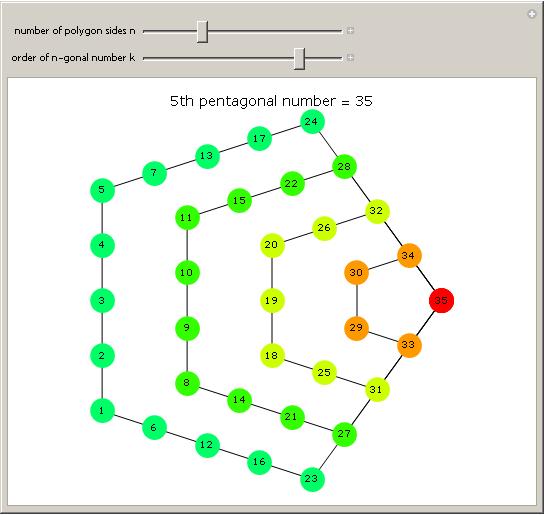
The 31st edition of the Carnival of Mathematics is up over at Recursivity. As always, there is a wide variety of material of offer with everything from recreational mathematics through to graduate level stuff. I liked the post on figurative numbers by Denise over at Let’s play math because I recently read about them in the book Recreations in the Theory of Numbers by Arthur Beiler. For a moment I thought it would be fun to write a Wolfram Demonstration about figurative numbers but it’s already been done – oh well, never mind. Enjoy the carnival.
In Matlab if you type the command
whos
then you will get a detailed list of all of the variables in the current workspace which is often very useful. The equivalent command in SAGE-Math is
show_identifiers()
I hope someone finds this useful.
In the recent 30th edition of the Carnival of Mathematics, the author mentioned that 30 is the first Sphenic number. I had never heard the term before so I thought I would investigate them a bit – nothing serious, just a bit of googling. The Wikipedia page was the first hit and this told me that Sphenic Numbers are positive integers that are the product of three distinct primes.
The article also demonstrated that Sphenic Numbers have exactly 8 divisors and gave some other bits of trivia such as the largest known example of a Sphenic Number (the product of the 3 largest known primes). There was also a link to the sequence of sphenic numbers on The On-Line Encyclopedia of Integer Sequences and that was about it. Oddly for something so elementary – there was nothing about Sphenic Numbers on Mathworld although this may change now that my Wolfram Demonstration on Sphenic Numbers has been published.
I was curious about what had written about Sphenic numbers in the literature so I googled the term on Google Scholar – amazingly there was not a single hit. So it seems that these numbers were considered important enough by someone to give them their own name but no one has then used that name in the literature….EVER!
How about books? Searching for “Sphenic Numbers” in Google Books also results in no hits. “Sphenic Number” results in one hit for a book called “Worlds of If” – No preview is available and the only quote you can get is “A sphenic number is one with unequal factors”
So – Where on earth did the name come from? Wikipedia says that its from the old greek word ‘sphen’ which means wedge but what I really want to know is who first gave these numbers this name? Why are there no references to the name in the literature? Does anyone know any interesting theorems concerning Sphenic Numbers?
Finally, is there a name for numbers that are the product of 4 distinct primes, or 5, or 6?
Abaqus is an extremely powerful finite element analysis (FEA) package that is used by various departments at my university and it is an application that I provide some of the support for among our users. I am far from being an expert at using it but I do know a trick or two and am occasionally useful. Recently, someone emailed me because they were having trouble actually getting Abaqus 6.6 installed on a 64 bit CENTOS 5 machine. He was located on the other side of campus from me, but it was a nice day and I felt like a walk so, rather than giving the support via email, I popped over to see him face to face. I am glad I did too – because it was a tricky one!
I am aware that this is not the sort of thing my usual readers might be interested in so I will keep it as brief as possible – basically what I want to do is provide myself with a permanent record of what we discovered and how we fixed it in case I come across this problem again. In an ideal world it might also help a googler or two (do let me know in the comments if it does – it will make my day)
So…we log on as root, run the installation script and get the following error
Extracting temporary installation utilities to /opt/temp…
Executing the installation GUI…
Preparing to install…
Extracting the installation resources from the installer archive…
Configuring the installer for this system’s environment…
awk: error while loading shared libraries: libdl.so.2: cannot open shared object file: No such file or directory
dirname: error while loading shared libraries: libc.so.6: cannot open shared object file: No such file or directory
/bin/ls: error while loading shared libraries: librt.so.1: cannot open shared object file: No such file or directory
basename: error while loading shared libraries: libc.so.6: cannot open shared object file: No such file or directory
dirname: error while loading shared libraries: libc.so.6: cannot open shared object file: No such file or directory
basename: error while loading shared libraries: libc.so.6: cannot open shared object file: No such file or directory
hostname: error while loading shared libraries: libc.so.6: cannot open shared object file: No such file or directory
Launching installer…
grep: error while loading shared libraries: libc.so.6: cannot open shared object file: No such file or directory
/opt/temp/TEMP_ABAQUS_utils_root/jre/bin/java: error while loading shared libraries: libpthread.so.0: cannot open shared object file: No such file or directory
As far as I can tell the reason for this is that the installer cannot identify your shiny new kernel so it assumes that an old one is being used and THIS is where the problems start. The problem occurs in the script /cdrom/lnx86_64/product/UNIX/Disk1/InstData/NoVM/install.bin
Look inside this file and you will see 2 lines that contain
export LD_ASSUME_KERNEL
I commented these out by adding a # (after copying the installation cd to a writable filesystem of course):
#export LD_ASSUME_KERNEL
BIG mistake. I now had a shiny new error
Exception in thread "main" java.lang.NoClassDefFoundError: com/zerog/lax/LAX
After a bit of googling, I discovered this post which gave an explanation of the problem along with a solution. The important part is this:
“make sure any line you put a comment on, you either edit in overwrite mode, or you make sure you delete a character for every # sign you add”
I deleted the Tab character before each of the # I had added and the error went away but I could have saved myself the grief by NOT manually commenting out each instance of LD_ASSUME_KERNEL and just running the following sed command on install.bin instead
cat install.bin | sed “s/export LD_ASSUME_KERNEL/#xport LD_ASSUME_KERNEL/” > /tmp/install.bin
Once this was taken care of, the installation proceeded without complaint and I was pretty confident that I was going to be out in time to meet my friend for coffee but, alas, it was not to be. When I tested the install by running the abaqus cae I received the following error message
/opt/abaqus/6.6-1/exec/ABQcaeK.exe: /opt/abaqus/6.6-1/External/libgcc_s.so.1: version `GCC_4.2.0′ not found (required by /usr/lib64/libstdc++.so.6)
I was starting to contemplate writing some FEA code for him rather than continue with this install as I felt that it might have been easier but it turned out that all we need to do is change the name of a couple of files (original source here). Do the following at your shell prompt (assuming the default installation location):
cd /opt/abaqus/6.6-1/External
mv libgcc_s.so libgcc_s.so.BACKUP
mv libgcc_s.so.1 libgcc_s.so.1.BACKUP
Job done! Finally! As always, if anyone finds this useful then please let me know.
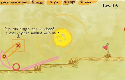
Almost immediately after posting about Crayon Physics and its Clones I had a message from a friend of mine who said “Crayon Physics is very cool!” – how right he was. Not long afterwards he sent another message “Check out Magic Pen” – so I did!
Magic Pen is a flash based game by Alejandro Guillen that is unashamedly a rip-off of inspired by Crayon Physics – the freeware physics-based game that has been a runaway success for its author, Petri Purho. They say that imitation is the best form of flattery and, looking at Magic Pen, Petri should be very flattered indeed.
I have already written quite a lot about this sort of game so I won’t go into details about the game mechanics – referring you instead to my original article. In some ways, Magic Pen surpasses Crayon Physics because it is a bit more flexible. For example, in Crayon Physics you can only draw blocks, but in Magic Pen you can also draw perfect circles and, additionally, produce more complicated structures with pins and hinges in them.
All in all its a great game that kept me happy for an hour or so but somehow it just doesn’t have quite the same charm as the original. This is not a major downfall though because the original has LOT of charm. Like many people, I am really waiting for Petri to release his sequel – Crayon Physics Deluxe – but in the meantime Magic Pen will do nicely.
In my attic there is an ancient computer desktop that is long past its sell by date and it is time to take it to the tip to be recycled. Before I do this though, I want to ensure that all of the data is securely removed from the hard drive. As many people know, just deleting the files is not enough as they will still be on the hard drive – your operating system will just pretend that they are not.
So what to do? Well, my solution was to use a Ubuntu Live CD to boot into Linux, open a terminal and issue the following command
shred -v -z /dev/hda
This wrote random data to the entire hard drive 25 times and then finished with a set of zeros. That’s pretty deleted!
I have heard that even with this level of ‘shredding’ it would still be possible for someone with suitable equipment (such as an AFM) and sufficient determination to get access to at least some of your old files but I am betting that such equipment is expensive and hard to obtain. I also can’t imagine why anyone would go to such lengths to view my old data – its not THAT interesting!
Essentially all I am trying to do here is stop the casual snooper from easily finding out what was on that hard disk and I think that the shred command does exactly that!
I am just about to go into hospital to have my wisdom teeth removed under general anesthetic, but before I go I thought I would mention that I have discovered an elementary proof of the Riemann Hypothesis and will share it with you all as soon as I get back.
Update – 11th April 2008
Of course I have not proved the Riemann Hypothesis at all but I was a bit worried about having that general anesthetic and so, following the example of Godfrey Harvey, I thought I would take out a little health insurance ;)
The minimization of the Rosenbrock function is a classic test problem that is extensively used to test the performance of different numerical optimization algorithms. It was first introduced in 1960 by H.H Rosenbrock in his paper, “An Automatic Method for Finding the Greatest or Least Value of a Function, Computer J. 3, 175-184, 1960 (See here for Rosenbrock’s account of how he came to write that paper.)
The function definition is given below and, although it looks harmless enough, it turns out to be quite challenging to find it’s minimum point by numerical methods.

Acording to Google Scholar, Rosenbrock’s paper has been cited no less than 596 times (as of April 9th 2008) and the function he introduced has been used as a test problem for many different numerical solvers including those in the Matlab Optimization toolbox, The NAG libraries, COMSOL and SciPy (A python module).
So why is this innocuous looking function so difficult to minimise? To answer that let’s first take a look at its contour plot using Mathematica.
ContourPlot[(1 – x)^2 + 100 (y – x^2)^2, {x, -2, 2}, {y, -2, 2},
ContourShading -> False, Contours -> Table[10^-i, {i, -2, 10, 0.5}]
, Epilog -> {Black, PointSize[Large], Point[{1, 1}]}]
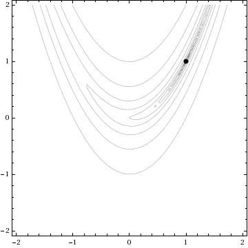
The global minimum of the Rosenbrock function lies at the point x=1, y=1 and is shown in the above diagram by a black spot. Note that the contours are not evenly spaced in this diagram – they are logarithmically spaced instead so the solution lies inside a very deep, narrow, banana shaped valley. The distinctive shape of this function’s contour lines is the reason for its alternative name – “Rosenbrock’s banana function”.
The valley causes a lot of problems for search algorithms such as the method of steepest descents which will quickly find the ‘entrance’ to the valley and then spend hundreds of iterations zigzagging from one side of it to the other – making very slow progress towards the minimum itself.
There is a Mathematica function called FindMinimum that can handle this kind of optimization problem and I wondered how its methods would handle the Rosenbrock function. In the back of my mind I thought that I might also be able to make a nice Wolfram Demonstration from the investigation. While looking at the documentation for FindMinimum I found an example that pretty much solved the problem for me.
pts = Reap[FindMinimum[(1 – x)^2 + 100 (-x^2 – y)^2, {{x, -1.2}, {y, 1}}, StepMonitor :> Sow[{x, y}]]][[2, 1]];
pts = Join[{{-1.2, 1}}, pts];
This finds the minimum point from a starting point of x=-1.2, y=1 and also stores all of the intermediate steps so you can see the path that Mathematica takes in looking for the solution. The only other piece of information needed was to find out how to specify the solution method. It turns out that this is obvious – just use the option
Method->”MethodNameHere”
replacing MethodNameHere with whatever method you want Mathematica to use. You can choose from ConjugateGradient, LevenbergMarquardt, Newton, QuasiNewton, PrincipalAxis and InteriorPoint.
All that remained was to wrap this up in a Manipulate statement, make it look pretty, add some controls and submit it to the demonstrations project. The result can be found here.
One of the things I like about the process of submitting demonstrations to the project is that they are refereed. Someone will take the time to look at your code and make suggestions and small modifications before it gets published. This reduces the possibility of mistakes being made in the final version and really helps with the learning process. Almost every time I have submitted something, I have learned a little more about Mathematica – and that’s really the main reason for me doing it (well its also fun to have your name “up in lights” if I am being honest).
At this point I would like to thank the members of the Wolfram Demonstrations team who have dealt with my submissions so far – not only have they been a pleasure to work with and extremely patient but they have also spared my blushes by pointing out some very stupid mistakes in my code. Of course any that remain are my fault and not theirs.
Interesting times lie ahead for Sage Math I think! This is definitely an application worth keeping an eye on.