
Archive for the ‘general math’ Category
The MATLAB community site, MATLAB Central, is celebrating its 20th anniversary with a coding competition where the only aim is to make an interesting image with under 280 characters of code. The 280 character limit ensures that the resulting code is tweetable. There are a couple of things I really like about the format of this competition, other than the obvious fact that the only aim is to make something pretty!
- No MATLAB license is required! Sign up for a free MathWorks account and away you go. You can edit and run code in the browser.
Stealingreusing other people’s code is actively encouraged! The competition calls it remixing but GitHub users will recognize it as forking.
Here’s an example. I wrote a piece of code to render the Sierpiński triangle – Wikipedia using a simple random algorithm called the Chaos game.
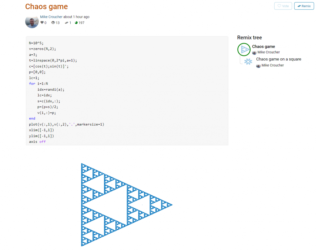
This is about as simple as the Chaos game gets and there are many things that could be done to produce a different image. As you can see from the Remix tree on the right hand side, I’ve already done one of them by changing a from 3 to 4 and adding some extra code to ensure that the same vertex doesn’t get chosen twice. This is result:
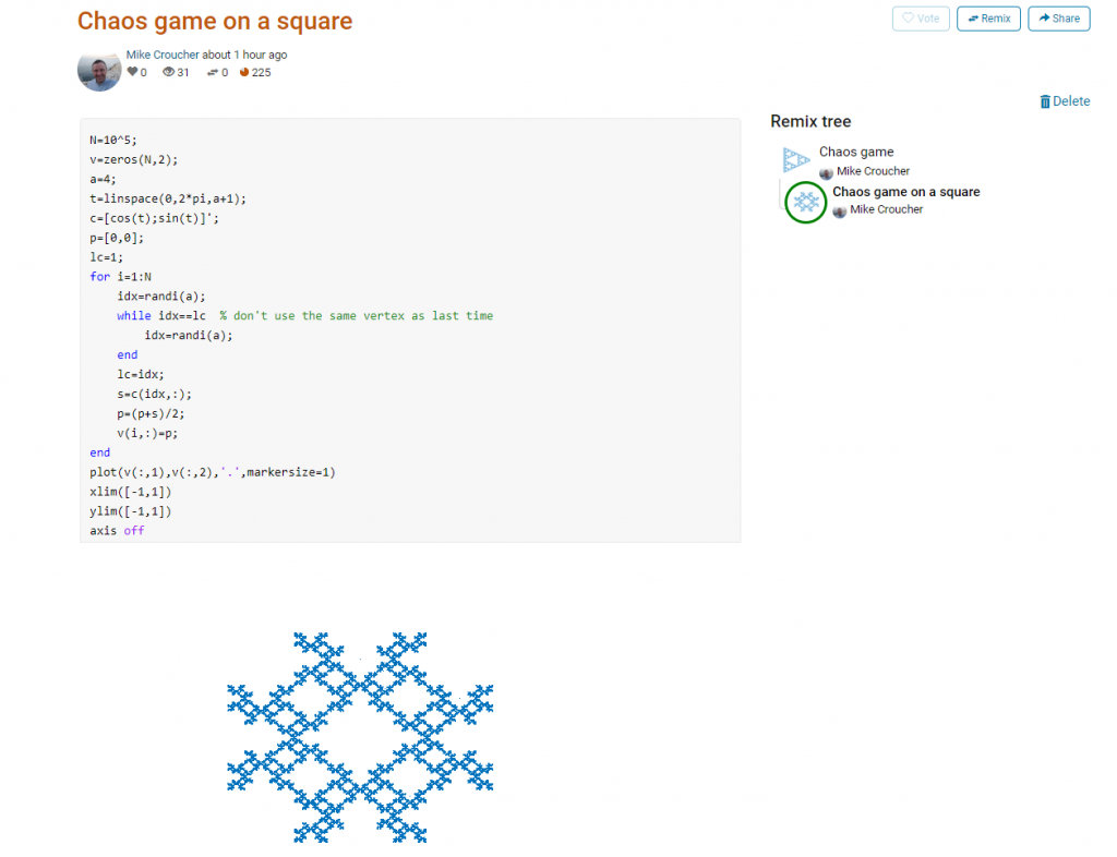
Someone else can now come along, hit the remix button and edit the code to produce something different again. Some things you might want to try for the chaos game include
- Try changing the value of a which is used in the variables t and c to produce the vertices of a polygon on an enclosing circle.
- Instead of just using the vertices of a polygon, try using the midpoints or another scheme for producing the attractor points completely.
- Try changing the scaling factor — currently p=(p+s)/2;
- Try putting limitations on which vertex is chosen. This remix ensures that the current vertex is different from the last one chosen.
- Each vertex is currently equally likely to be chosen using the code idx=randi(a); Think of ways to change the probabilities.
- Think of ways to colorize the plots.
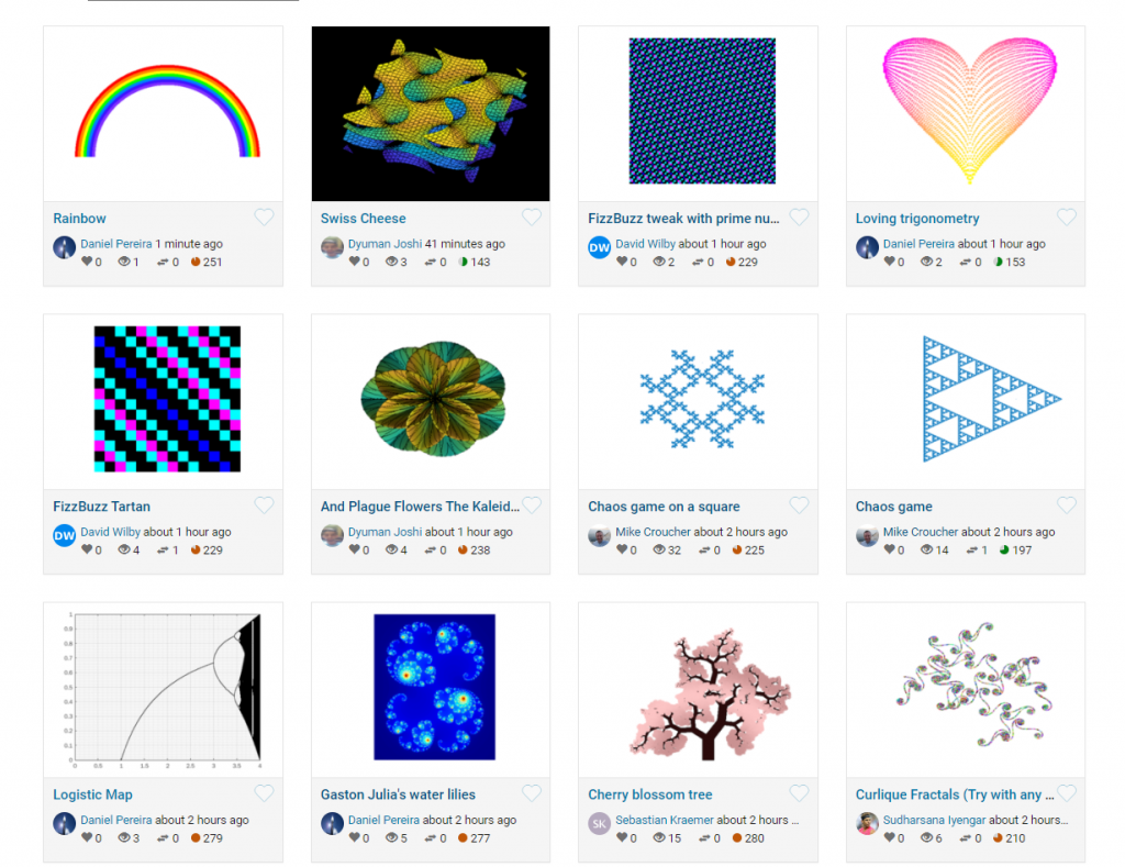
Maybe the chaos game isn’t your thing. You are free to create your own design from scratch or perhaps you’d prefer to remix some of the other designs in the gallery.
The competition is just a few hours old and there are already some very nice ideas coming out.
I was in a funk!
Not long after joining the University of Sheffield, I had helped convince a raft of lecturers to switch to using the Jupyter notebook for their lecturing. It was an easy piece of salesmanship and a whole lot of fun to do. Lots of people were excited by the possibilities.
The problem was that the University managed desktop was incapable of supporting an instance of the notebook with all of the bells and whistles included. As a cohort, we needed support for Python 2 and 3 kernels as well as R and even Julia. The R install needed dozens of packages and support for bioconductor. We needed LateX support to allow export to pdf and so on. We also needed to keep up to date because Jupyter development moves pretty fast! When all of this was fed into the managed desktop packaging machinery, it died. They could give us a limited, basic install but not one with batteries included.
I wanted those batteries!
In the early days, I resorted to strange stuff to get through the classes but it wasn’t sustainable. I needed a miracle to help me deliver some of the promises I had made.
Miracle delivered – SageMathCloud
During the kick-off meeting of the OpenDreamKit project, someone introduced SageMathCloud to the group. This thing had everything I needed and then some! During that presentation, I could see that SageMathCloud would solve all of our deployment woes as well as providing some very cool stuff that simply wasn’t available elsewhere. One killer-application, for example, was Google-docs-like collaborative editing of Jupyter notebooks.
I fired off a couple of emails to the lecturers I was supporting (“Everything’s going to be fine! Trust me!”) and started to learn how to use the system to support a course. I fired off dozens of emails to SageMathCloud’s excellent support team and started working with Dr Marta Milo on getting her Bioinformatics course material ready to go.
TL; DR: The course was a great success and a huge part of that success was the SageMathCloud platform
Giving back – A tutorial for lecturers on using SageMathCloud
I’m currently working on a tutorial for lecturers and teachers on how to use SageMathCloud to support a course. The material is licensed CC-BY and is available at https://github.com/mikecroucher/SMC_tutorial
If you find it useful, please let me know. Comments and Pull Requests are welcome.
Some numbers have something to say. Take the following, rather huge number, for example:
185325291040682644803531312384041336595151018761127807725763308064246070395230764956468856341399670487
514610052487586323067575687914642829757636555138456145938430191876551756992329818006401775522301219016
237245425891544032218544390861818271526845858747648909382915665997160517028671058273052955697138350617
856171748990490346558484883522495310587304606877332488244886849690319641412147118669050542398759303832
627672479768452329971883073420877438596419179762421854464516060347269129680634374662501202129049727949
71185874579656679344857677824
This number wants to tell you ‘Happy Holidays’, it just needs a little code to help it out. In Maple, this code is:
n := 18532529104068264480353131238404133659515101876112780772576330806424607039523076495646885634139967048751461005248758632306757568791464282975763655513845614593843019187655175699232981800640177552230121901623724542589154403221854439086181827152684585874764890938291566599716051702867105827305295569713835061785617174899049034655848488352249531058730460687733248824488684969031964141214711866905054239875930383262767247976845232997188307342087743859641917976242185446451606034726912968063437466250120212904972794971185874579656679344857677824:
modnew := proc (x, y) options operator, arrow; x-y*floor(x/y) end proc:
tupper := piecewise(1/2 < floor(modnew(floor((1/17)*y)*2^(-17*floor(x)-modnew(floor(y), 17)), 2)), 0, 1):
points := [seq([seq(tupper(x, y), y = n+16 .. n, -1)], x = 105 .. 0, -1)]:
plots:-listdensityplot(points, scaling = constrained, view = [0 .. 106, 0 .. 17], style = patchnogrid, size = [800, 800]);
The result is the following plot

Thanks to Samir for this one!
The mathematics is based on a generalisation of Tupper’s self-referential formula.
There’s more than one way to send a message with an equation, however. Here’s an image of one I discovered a few years ago — The equation that says Hi

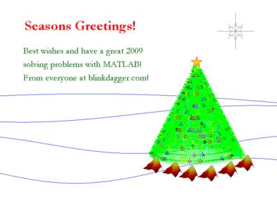
Way back in 2008, I wrote a few blog posts about using mathematical software to generate christmas cards:
- Mathematical Christmas Cards – Walking Randomly Christmas Challenge
- A MATLAB Christmas card
- Christmas geetings – SAGE style
I’ve started moving the code from these to a github repository. If you’ve never contributed to an open source project before and want some practice using git or github, feel free to write some code for a christmas message along similar lines and submit a Pull Request.
Given a symmetric matrix such as
![\light \[ \left( \begin{array}{ccc} 1 & 1 & 0 \\ 1 & 1 & 1 \\ 0 & 1 & 1 \end{array} \right)\]](https://walkingrandomly.com/wp-content/ql-cache/quicklatex.com-0ba648b6b45c6e624aefe7341a911896_l3.png "Rendered by QuickLaTeX.com")
What’s the nearest correlation matrix? A 2002 paper by Manchester University’s Nick Higham which answered this question has turned out to be rather popular! At the time of writing, Google tells me that it’s been cited 394 times.
Last year, Nick wrote a blog post about the algorithm he used and included some MATLAB code. He also included links to applications of this algorithm and implementations of various NCM algorithms in languages such as MATLAB, R and SAS as well as details of the superb commercial implementation by The Numerical algorithms group.
I noticed that there was no Python implementation of Nick’s code so I ported it myself.
Here’s an example IPython session using the module
In [1]: from nearest_correlation import nearcorr

In [2]: import numpy as np

In [3]: A = np.array([[2, -1, 0, 0],
   ...:               [-1, 2, -1, 0],
   ...:               [0, -1, 2, -1],
   ...:               [0, 0, -1, 2]])

In [4]: X = nearcorr(A)

In [5]: X
Out[5]:
array([[ 1.        , -0.8084125 ,  0.1915875 ,  0.10677505],
       [-0.8084125 ,  1.        , -0.65623269,  0.1915875 ],
       [ 0.1915875 , -0.65623269,  1.        , -0.8084125 ],
       [ 0.10677505,  0.1915875 , -0.8084125 ,  1.        ]])
This module is in the early stages and there is a lot of work to be done. For example, I’d like to include a lot more examples in the test suite, add support for the commercial routines from NAG and implement other algorithms such as the one by Qi and Sun among other things.
Hopefully, however, it is just good enough to be useful to someone. Help yourself and let me know if there are any problems. Thanks to Vedran Sego for many useful comments and suggestions.
- github repository for the Python NCM module, nearest_correlation
- Nick Higham’s original MATLAB code.
- NAG’s commercial implementation – callable from C, Fortran, MATLAB, Python and more. A superb implementation that is significantly faster and more robust than this one!
A recent Google+ post from Mathemania4u caught my attention on the train to work this morning. I just had to code up something that looked like this and so fired up Mathematica and hacked away. The resulting notebook can be downloaded here. It’s not particularly well thought through so could almost certainly be improved on in many ways.
The end result was a Manipulate which you’ll be able to play with below, provided you have a compatible Operating System and Web browser. The code for the Manipulate is
Manipulate[
 Graphics[Map[dotCirc,
   circArray[circrad, theta, pointsize, extent, step, phase,
    showcirc]]]
 , {{showcirc, True, "Show Circles"}, {True, False}}
 , {{theta, 0, "Dot Angle"}, 0, 2 Pi, Pi/10, Appearance -> "Labeled"}
 , {{pointsize, 0.018, "Dot Size"}, 0, 1, Appearance -> "Labeled"}
 , {{phase, 2, "Phase Diff"}, 0, 2 Pi, Appearance -> "Labeled"}
 , {{step, 0.25, "Circle Separation"}, 0, 1, Appearance -> "Labeled"}
 , {{extent, 2, "Plot Extent"}, 1, 5, Appearance -> "Labeled"}
 , {{circrad, 0.15, "Circle Radius"}, 0.01, 1, Appearance -> "Labeled"}
 , Initialization :>
  {
   dotCirc[{x_, y_, r_, theta_, pointsize_, showcirc_}] := If[showcirc,
     {Circle[{x, y}, r], PointSize[pointsize],
      Point[{x + r Cos[theta], y + r Sin[theta]}]}
     ,
     {PointSize[pointsize],
      Point[{x + r Cos[theta], y + r Sin[theta]}]}]
   ,
   circArray[r_, theta_, pointsize_, extent_, step_, phase_,
     showcirc_] := Module[{},
     Partition[
      Flatten[Table[{x, y, r, theta + x*phase + y*phase, pointsize,
         showcirc}, {x, -extent, extent, step}, {y, -extent, extent,
         step}]], 6]
     ]}]
If you can use the Manipulate below, I suggest clicking on the + icon to the right of the ‘Dot Angle’ field to expose the player controls and then press the play button to kick off the animation.
I also produced a video – The code used to produce this is in the notebook.
)
A lot of people don’t seem to know this….and they should. When working with floating point arithmetic, it is not necessarily true that a+(b+c) = (a+b)+c. Here is a demo using MATLAB
>> x=0.1+(0.2+0.3);
>> y=(0.1+0.2)+0.3;
>> % are they equal?
>> x==y

ans =
     0

>> % lets look
>> sprintf('%.17f',x)
ans =
0.59999999999999998

>> sprintf('%.17f',y)
ans =
0.60000000000000009
These results have nothing to do with the fact that I am using MATLAB. Here’s the same thing in Python
>>> x=(0.1+0.2)+0.3
>>> y=0.1+(0.2+0.3)
>>> x==y
False
>>> print('%.17f' %x)
0.60000000000000009
>>> print('%.17f' %y)
0.59999999999999998
If this upsets you, or if you don’t understand why, I suggest you read the following
Does anyone else out there have suggestions for similar resources on this topic?
In a recent blog-post, John Cook, considered when series such as the following converged for a given complex number z
z1 = sin(z)
z2 = sin(sin(z))
z3 = sin(sin(sin(z)))
John’s article discussed a theorem that answered the question for a few special cases and this got me thinking: What would the complete set of solutions look like? Since I was halfway through my commute to work and had nothing better to do, I thought I’d find out.
The following Mathematica code considers points in the square portion of the complex plane where both real and imaginary parts range from -8 to 8. If the sequence converges for a particular point, I colour it black.
LaunchKernels[4]; (*Set up for 4 core parallel compute*)
ParallelEvaluate[SetSystemOptions["CatchMachineUnderflow" -> False]];
convTest[z_, tol_, max_] := Module[{list},
  list = Quiet[
    NestWhileList[Sin[#] &, z, (Abs[#1 - #2] > tol &), 2, max]];
  If[
   Length[list] < max && NumericQ[list[[-1]]]
   , 1, 0]
  ]
step = 0.005;
extent = 8;
AbsoluteTiming[
 data = ParallelMap[convTest[#, 10*10^-4, 1000] &,
    Table[x + I y, {y, -extent, extent, step}, {x, -extent, extent,
      step}]
    , {2}];]
ArrayPlot[data]
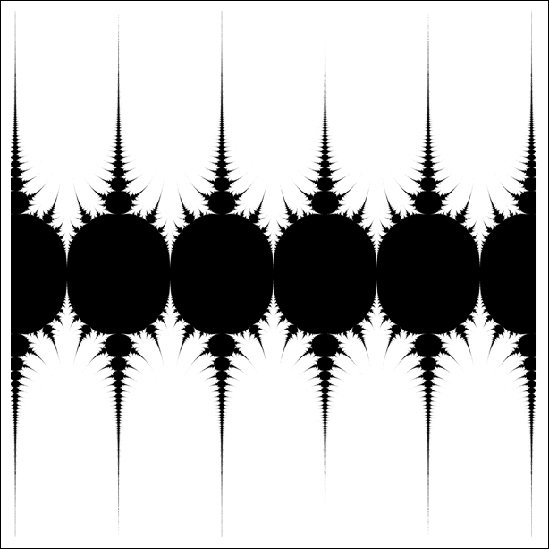
I quickly emailed John to tell him of my discovery but on actually getting to work I discovered that the above fractal is actually very well known. There’s even a colour version on Wolfram’s MathWorld site. Still, it was a fun discovery while it lasted
Other WalkingRandomly posts like this one:
The University of Manchester has uploaded some videos of Cornelius Lanczos the (re-)discoverer of the fast Fourier transform and singular value decomposition among other things. Recorded back in 1972, these videos discuss his life and mathematics. Worth taking a look.
Update: Manchester’s Nick Higham has written a more detailed blog post about these videos – http://nickhigham.wordpress.com/2013/02/06/the-lanczos-tapes/
While on the train to work I came across a very interesting blog entry. Full LaTeX support (on device compilation and .dvi viewer) is now available on iPad courtesy of TeX Writer By FastIntelligence. Here is the blog post telling us the good news http://litchie.com/blog/?p=406
At the time of writing, the blog is down (Update: working again), possibly because of the click storm that my twitter announcement caused..especially after it was picked up by @TeXtip. So, here is the iTunes link http://itunes.apple.com/us/app/tex-writer/id552717222?mt=8
I haven’t tried this yet but it looks VERY interesting. If you get a chance to try it out, feel free to let me know how you get on in the comments section.
Update 1: This version of TeX writer(1.1) cannot output to .pdf. Only .dvi output is supported at the moment.