
Archive for the ‘programming’ Category
The student version of MATLAB is a bargain since it only costs $99 (or less than £50 for those of us in the UK) and it comes complete with several toolboxes including symbolic maths, statistics and optimisation. Most of it is identical to the full academic version which would cost well over a thousand pounds if you bought all of the toolboxes included in the student version. The only place where it is ‘crippled’ is within Simulink since your Simulink models are limited to 1000 blocks. There are one or two other differences too and I refer you to the amazon page
for full details (Amazon is also the cheapest place I could find for Student MATLAB by the way).
One problem with the student version of MATLAB though is the fact that they only supply a 32 bit version. This was potentially a big problem for a friend of mine since he has a 64bit Linux machine with 4Gb of RAM. Fortunately, the 32bit version installs OK on 64bit Linux but the result is completely unsupported by Mathworks. Fair enough….It works and he is (mostly) happy since he gets a lot of functionality for his money.
One thing that definitely didn’t work though was compiling mex files. No matter how hard we tried we simply could not get it to work which made me look bad because I am supposed to be ‘The MATLAB guy’ around here. Well, sometimes it’s not what you know but who you know that counts and I know a LOT of MATLAB users. One of them has provided a fix but doesn’t want his name plastered all over Walking Randomly. So, thanks to Mr Anonymous we got mex files working on Student MATLAB 2009a running on 64bit Linux and this is how we did it.
Get a simple mex file and try to compile it. You’ll probably get this error.
/usr/bin/ld: cannot find -lmx
The way to get around that is to run the following command in MATLAB just before you try to compile a mex file
setenv('MATLAB_ARCH', 'glnx86') (IN MATLAB)
That gets you a little further but you’ll next be hit by
/usr/bin/ld: cannot find -lstdc++
To fix this you need to find your mexopts.sh file and change the line
CLIBS="$CLIBS -lstdc++"
to
CLIBS="$CLIBS -L/home/paul/matlab/R2009a-student/sys/os/glnx86 -lstdc++"
obviously, you’ll need to change /home/paul/matlab to wherever you actually installed MATLAB.
Your next step is to do the following in a bash prompt
ln -s /home/paul/matlab/R2009a-student/sys/os/glnx86/libstdc++.so.6 \
/home/paul/matlab/R2009a-student/sys/os/glnx86/libstdc++.so
again – substituting wherever you installed MATLAB for /home/paul/matlab
Paul was running Ubuntu 9.04 and he got the following error at some point (I can’t remember where)
/usr/include/gnu/stubs.h:7:27: error: gnu/stubs-32.h: No such file or directory
which was fixed by
sudo apt-get install libc6-dev-i386
That’s pretty much it. You should now be able to compile mex files. Hope this helps someone out there.
In order to write fully parallel programs in MATLAB you have a few choices but they are either hard work, expensive or both. For example you could
- Write parallel mex files using C and OpenMP
- Drop a load of cash on the parallel computing toolbox from the Mathworks
- Use the free parallel toolbox, pMATLAB
Wouldn’t it be nice if you could do no work at all and yet STILL get a speedup on a multicore machine? Well, you can….sometimes.
Slowly but surely, The Mathworks are parallelising some of the built in MATLAB functions to make use of modern multicore processors. So, for certain functions you will see a speed increase in your code when you move to a dual or quad core machine. But which functions?
On a recent train journey I trawled through all of the release notes in MATLAB and did my best to come up with a definitive list and the result is below.
Alongside each function is the version of MATLAB where it first became parallelised (if known). If there is any extra detail then I have included it in brackets (typically things like – ‘this function is only run in parallel for input arrays of more than 20,000 elements’). I am almost certainly missing some functions and details so if you know something that I don’t then please drop me a comment and I’ll add it to the list.
Of course when I came to write all of this up I did some googling and discovered that The Mathworks have already answered this question themselves! Oh well….I’ll publish my list anyway.
Update 11th May 2012 While optimising a user’s application, I discovered that the pinv function makes use of multicore processors so I’ve added it to the list. pinv makes use of svd which is probably the bit that’s multithreaded.
Update 18th February 2012: Added a few functions that I had missed earlier: erfcinv, rank,isfinite,lu and schur. Not sure when they became multithreaded so left the version number blank for now
Update 16th June 2011: Added new functions that became multicore aware in version 2011a plus a couple that have been multicore for a while but I just didn’t know about them!
Update 8th March 2010: Added new functions that became multicore aware in version 2010a. Also added multicore aware functions from the image processing toolbox.
abs (for double arrays > 200k elements),2007a
acos (for double arrays > 20k elements),2007a
acosh (for double arrays > 20k elements),2007a
applylut,2009b (Image processing toolbox)
asin (for double arrays > 20k elements),2007a
asinh(for double arrays > 20k elements),2007a
atan (for double arrays > 20k elements),2007a
atand (for double arrays > 20k elements),2007a
atanh (for double arrays > 20k elements),2007a
backslash operator (A\b for double arrays > 40k elements),2007a
bsxfun,2009b
bwmorph,2010a (Image processing toolbox)
bwpack,2009b (Image processing toolbox)
bwunpack,2009b (Image processing toolbox)
ceil (for double arrays > 200k elements),2007a
conv,2011a
conv2,(two input form),2010a
cos (for double arrays > 20k elements),2007a
cosh (for double arrays > 20k elements),2007a
det (for double arrays > 40k elements),2007a
edge,2010a (Image processing toolbox)
eig
erf,2009b
erfc,2009b
erfcinv
erfcx,2009b
erfinv,2009b
exp (for double arrays > 20k elements),2007a
expm (for double arrays > 40k elements),2007a
fft,2009a
fft2,2009a
fftn,2009a
filter,2009b
fix (for double arrays > 200k elements),2007a
floor (for double arrays > 200k elements),2007a
gamma,2009b
gammaln,2009b
hess (for double arrays > 40k elements),2007a
hypot (for double arrays > 200k elements),2007a
ifft,2009a
ifft2,2009a
ifftn,2009a
imabsdiff,2010a (Image processing toolbox)
imadd,2010a (Image processing toolbox)
imclose,2010a (Image processing toolbox)
imdilate,2009b (Image processing toolbox)
imdivide,2010a (Image processing toolbox)
imerode,2009b (Image processing toolbox)
immultiply,2010a (Image processing toolbox)
imopen,2010a (Image processing toolbox)
imreconstruct,2009b (Image processing toolbox)
int16 (for double arrays > 200k elements),2007a
int32 (for double arrays > 200k elements),2007a
int8 (for double arrays > 200k elements),2007a
inv (for double arrays > 40k elements),2007a
iradon,2010a (Image processing toolbox)
isfinite
isinf (for double arrays > 200k elements),2007a
isnan (for double arrays > 200k elements),2007a
ldivide,2008a
linsolve (for double arrays > 40k elements),2007a
log,2008a
log2,2008a
logical (for double arrays > 200k elements),2007a
lscov (for double arrays > 40k elements),2007a
lu
Matrix Multiply (X*Y - for double arrays > 40k elements),2007a
Matrix Power (X^N - for double arrays > 40k elements),2007a
max (for double arrays > 40k elements),2009a
medfilt2,2010a (Image processing toolbox)
min (for double arrays > 40k elements),2009a
mldivide (for sparse matrix input),2009b
mod (for double arrays > 200k elements),2007a
pinv
pow2 (for double arrays > 20k elements),2007a
prod (for double arrays > 40k elements),2009a
qr (for sparse matrix input),2009b
qz,2011a
rank
rcond (for double arrays > 40k elements),2007a
rdivide,2008a
rem,2008a
round (for double arrays > 200k elements),2007a
schur
sin (for double arrays > 20k elements),2007a
sinh (for double arrays > 20k elements),2007a
sort (for long matrices),2009b
sqrt (for double arrays > 20k elements),2007a
sum (for double arrays > 40k elements),2009a
svd,
tan (for double arrays > 20k elements),2007a
tand (for double arrays > 200k elements),2007a
tanh (for double arrays > 20k elements),2007a
unwrap (for double arrays > 200k elements),2007a
various operators such as x.^y (for double arrays > 20k elements),2007a
Integer conversion and arithmetic,2010a
Earlier today I was chatting to a lecturer over coffee about various mathematical packages that he might use for an upcoming Masters course (note – offer me food or drink and I’m happy to talk about pretty much anything). He was mainly interested in Mathematica and so we spent most of our time discussing that but it is part of my job to make sure that he considers all of the alternatives – both commercial and open source. The course he was planning on running (which I’ll keep to myself out of respect for his confidentiality) was definitely a good fit for Mathematica but I felt that SAGE might suite him nicely as well.
“Does it have nice, interactive functionality like Mathematica’s Manipulate function?” he asked
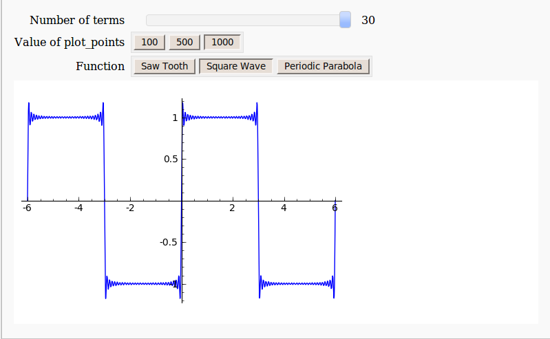
Oh yes! Here is a toy example that I coded up in about the same amount of time that it took to write the introductory paragraph above (but hopefully it has no mistakes). With just a bit of effort pretty much anyone can make fully interactive mathematical demonstrations using completely free software. For more examples of SAGE’s interactive functionality check out their wiki.
Here’s the code:
def ftermSquare(n):
 return(1/n*sin(n*x*pi/3))

def ftermSawtooth(n):
 return(1/n*sin(n*x*pi/3))

def ftermParabola(n):
 return((-1)^n/n^2 * cos(n*x))

def fseriesSquare(n):
 return(4/pi*sum(ftermSquare(i) for i in range (1,2*n,2)))

def fseriesSawtooth(n):
 return(1/2-1/pi*sum(ftermSawtooth(i) for i in range (1,n)))

def fseriesParabola(n):
 return(pi^2/3 + 4*sum(ftermParabola(i) for i in range(1,n)))

@interact
def plotFourier(n=slider(1, 30,1,10,'Number of terms')
,plotpoints=('Value of plot_points',[100,500,1000]),Function=['Saw Tooth','Square Wave','Periodic Parabola']):
    if Function=='Saw Tooth':
     show(plot(fseriesSawtooth(n),x,-6,6,plot_points=plotpoints))
    if Function=='Square Wave':
     show(plot(fseriesSquare(n),x,-6,6,plot_points=plotpoints))
    if Function=='Periodic Parabola':
     show(plot(fseriesParabola(n),x,-6,6,plot_points=plotpoints))
Almost every computer you buy these days contains more than one processor core – even my laptop has 2 – and I have access to relatively inexpensive desktops that have as many as 8. So, it is hardly surprising that I am steadily receiving more and more queries from people interested in making their calculations run over as many simultaneous cores as possible.
The big three Ms of the mathematical software world, Mathematica, Maple and MATLAB, all allow you to explicitly parallelise your own programs (although you have to pay extra if you want to do this in MATLAB without resorting to hand crafted C-code) but parallel programming isn’t easy and so tutorials are invaluable.
Fortunately, Darin Ohashi, a senior kernel developer at Maplesoft has taken the time to write some parallel Maple tutorials for us and he has presented his work as a series of blog posts over at MaplePrime. Here’s an idex:
- The Parallel Programming Blog
- Why Go Parallel?
- What Makes Parallel Programming Hard?
- Thread Safety
- Load Balancing and Thread Management
- The Task Programming Model
- Parallel Programming Blog Feedback
If you are interested in parallel programming in Maple then Darin’s posts are a great place to start.
Other articles from Walking Randomly you may be interested in
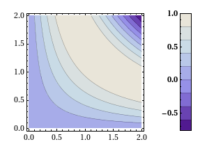
Will Robertson and I have released a new version of our colorbarplot package for Mathematica 6 and above. Colorbarplot has only one aim and that is to allow Mathematica users to add a MATLAB-like colorbar to their graphs. Something like this for example:

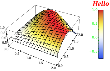
Version 0.5 is a very small upgrade from 0.4 in that it allows you to change the font style of the colorbar ticks as well as it’s label – as requested by Murat Havzalı. Here are a couple of examples of the new functionality:
ColorbarPlot[Sin[#1 #2] &, {0, 2}, {0, 2},
 PlotType -> "Contour",
 CTicksStyle -> Bold]
ColorbarPlot[Sin[#1 #2] &, {0, 2}, {0, 2},
 PlotType -> "3D",
 CLabel -> "Hello",
 ColorFunction -> "TemperatureMap",
 CLabelStyle -> Directive[Red, Italic, Bold, FontSize -> 20],
 CTicksStyle -> Directive[Green, FontFamily -> "Helvetica"]
 ]
Colorbarplot comes with an extensive examples file and you can download version 0.5 either from me or from Will’s github repository. We hope you find it useful and comments are welcomed.
- UPDATE 12th Novermber 2010. Update to version 0.6
Slowly but surely more and more MATLAB functions are becoming able to take advantage of multi-core processors. For example, in MATLAB 2009b, functions such as sort, bsxfun, filter and erf (among others) gained the ability to spread the calculational load across several processor cores. This is good news because if your code uses these functions, and if you have a multi-core processor, then you will get faster execution times without having to modify your program. This kind of parallelism is called implicit parallelism because it doesn’t require any special commands in order to take advantage of multiple cores – MATLAB just does it automagically. Faster code for free!
For many people though, this isn’t enough and they find themselves needing to use explicit parallelism where it becomes the programmer’s responsibility to tell MATLAB exactly how to spread the work between the multiple processing cores available. The standard way of doing this in MATLAB is to use the Parallel Computing Toolbox but, unlike packages such as Mathematica and Maple, this functionality is going to cost you extra.
There is another way though…
I’ve recently been working with David Szotten, a postgraduate student at Manchester University, on writing parallel mex files for MATLAB using openmp and C. Granted, it’s not as easy as using the Parallel Computing Toolbox but it does work and the results can be blisteringly fast since we are working in C. It’s also not quite as difficult as we originally thought it might be.
There is one golden rule you need to observe:
Never, ever call any of the mex api functions inside the portion of your code that you are trying to parallelise using openmp. Don’t try to interact with MATLAB at all during the parallel portion of your code.
The reason for the golden rule is because, at the time of writing at least (MATLAB 2009b), all mex api functions are not thread-safe and that includes the printf function since printf is defined to be mexPrintf in the mex.h header file. Stick to the golden rule and you’ll be fine. Move away from the golden rule,however, and you’ll find dragons. Trust me on this!
Let’s start with an example and find the sum of foo(x) where foo is a moderately complicated function and x is a large number of values. We have implemented such an example in the mex function mex_sum_openmp.
I assume you are running MATLAB 2009b on 32bit Ubuntu Linux version 9.04 – just like me. If your setup differs from this then you may need to modify the following instructions accordingly.
- Before you start. Close all currently running instances of MATLAB.
- Download and unzip the file mex_sum_openmp.zip to give you mex_sum_openmp.c
- Open up a bash terminal and enter export OMP_NUM_THREADS=2 (replace 2 with however many cores your machine has)
- start MATLAB from this terminal by entering matlab.
- Inside MATLAB, navigate to the directory containing mex_sum_openmp.c
- Inside MATLAB, enter the following to compile the .c file
mex mex_sum_openmp.c CFLAGS="\$CFLAGS -fopenmp" LDFLAGS="\$LDFLAGS -fopenmp"
- Inside MATLAB, test the code by entering
x=rand(1,9999999); %create an array of random x values
mex_sum_openmp(x) %calculate the sum of foo(x(i))
- If all goes well, this calculation will be done in parallel and you will be rewarded with a single number. Time the calculation as follows.
tic;mex_sum_openmp(x);toc
- My dual core laptop did this in about 0.6 seconds on average. To see how much faster this is compared to single core mode just repeat all of the steps above but start off with export OMP_NUM_THREADS=1 (You won’t need to recompile the mex function). On doing this, my laptop did it in 1.17 seconds and so the 2 core mode is almost exactly 2 times faster.
Let’s take a look at the code.
#include "mex.h"
#include <math.h>
#include <omp.h>

double spawn_threads(double x[],int cols)
{
	double sum=0;
	int count;
        #pragma omp parallel for shared(x, cols) private(count) reduction(+: sum)
	for(count = 0;count<cols;count++)
	{
	     sum += sin(x[count]*x[count]*x[count])/cos(x[count]+1.0);;
	}

	return sum;
}

void mexFunction(int nlhs,mxArray* plhs[], int nrhs, const mxArray* prhs[])
{
	double sum;
	 /* Check for proper number of arguments. */
 	if(nrhs!=1) {
    	mexErrMsgTxt("One input required.");
  	} else if(nlhs>1) {
    	mexErrMsgTxt("Too many output arguments.");
  	}

	/*Find number of rows and columns in input data*/
	int rows = mxGetM(prhs[0]);
	int cols = mxGetN(prhs[0]);

	/*I'm only going to consider row matrices in this code so ensure that rows isn't more than 1*/
	if(rows>1){
	mexErrMsgTxt("Input data has too many Rows.  Just the one please");
	}

	/*Get pointer to input data*/
	double* x = mxGetPr(prhs[0]);

	/*Do the calculation*/
	sum = spawn_threads(x,cols);

	/*create space for output*/
 	 plhs[0] = mxCreateDoubleMatrix(1,1, mxREAL);

	/*Get pointer to output array*/
	double* y = mxGetPr(plhs[0]);

	/*Return sum to output array*/
	y[0]=sum;

}
That’s pretty much it – the golden rule in action. I hope you find this example useful and thanks again to David Szotten who helped me figure all of this out. Comments welcomed.
Other articles you may find useful
- MATLAB mex functions using the NAG C Library in Windows – This article includes an OpenMP example compiled on Visual Studio 2008 in Windows.
If you have learned how to program then the odds are that you have written a program that displays a list of prime numbers. A prime number generator is a programming rite of passage that is almost up there with the ubiquitous ‘Hello World‘ application (for programmers who are going on to do numerical work at least).
There are various ways you might choose to do it but I bet that your first (or even your second or third) thought wouldn’t be ‘I know – I’ll use a regular expression‘. Someone known only as ‘Abigail’ obviously thought that the world desperately needed such a regex since he / she came up with the following incantation
^1?$|^(11+?)\1+$
Which is a regular expression that I assure you can be used to generate a list of all the prime numbers. If you are in the mood for a puzzle then sit back, grab a cup of coffee and try to work out HOW it can generate the primes.
If you give up then head over to Python Programming for a full explanation along with Python code that demonstrates that it really does work.
Can anyone come up with regular expressions for other interesting series of numbers?
Update (27th August 2009): Someone pointed me to an alternative explanation here.
The latest version of NAG’s toolbox for MATAB has been released for Linux users (Windows versions will follow at a later date) and is available for download over at NAG’s website.
This release syncs the MATLAB toolbox up with Mark 22 of the NAG Fortran library and there is a lot of interesting new functionality including:
- Global Optimisation
- Wavelets
- ProMax rotations
- Improved Sobol quasi random number generator (good for up to 50000 dimensions)
- Option Pricing Formulae
- Lambert’s W function
- A fast quantile routine
- Matrix exponentials
I really like the NAG toolbox for MATLAB for the following reasons (among others):
- It has saved my employer, The University of Manchester, a lot of money since we don’t need as many licenses for toolboxes such as Statistics, Optimisation, Curve Fitting and Splines.
- It can speed up MATLAB calculations – see my article on MATLAB’s interp1 function for example
- It has some functionality that can’t be found in MATLAB.
- Their support team is superb.
Although written for the previous version of the NAG Toolbox for MATLAB, the following articles will be useful for anyone who wants to get started with the toolbox.
- Calling the NAG routines from MATLAB
- Using the NAG Toolbox for MATLAB part 1
- Using the NAG Toolbox for MATLAB part 2
- Using the NAG Toolbox for MATLAB part 3
Previous articles written by me about the NAG toolbox for MATLAB include
- NAG – The ultimate toolbox for MATLAB (a write up of Mark 21 of the toolbox)
- A faster version of MATLAB’s interp1 (How I helped a user drastically speed up her code by swapping MATLAB’s interp 1 function with a couple from the NAG toolbox – real world code runtime reduced from 1hour 10mins per run down to 26mins per run)
One of the things I love most about blogging is the interaction with readers via the comments section. Put simply you guys know your onions and although I (hopefully) have something useful and/or interesting to tell you, there is a heck of a lot of stuff that you could tell me.
In the comments section of one of my recent posts, Sander Huisman, did exactly that when he suggested that I shouldn’t always use Table in Mathematica when generating lists. This was news to me – I thought that Table was the accepted and possibly the fastest way to do it in Mathematica but it seems not. Here is a concrete example as provided by Sander.
AbsoluteTiming[Table[PrimeQ[i], {i, 0, 10000000}];]
AbsoluteTiming[PrimeQ /@ Range[0, 10000000];]
Both of these Mathematica expressions test each of the first 10000000 integers (including 0) to see if they are prime and what you end up with is a list of Booleans – {False, False, True, True, False, True, False, True, False, False} and so on. The difference is that the first expression is noticeably slower than the second.
If, like me, you struggle to remember what the punctuation operators (/. /@ etc) actually do in Mathematica then know that foo /@ bar is equivalent to Map[foo,bar] where foo is a funbction and bar is a list.
On one of my test machines, the first expression evaluated in 10.012 seconds on average whereas the second evaluated in 8.28 seconds on average (both averages are over 100 runs).
So Map is faster than Table right?
Maybe, maybe not. Try the following examples (again provided by Sander) where we generate a list of i+2 for i between 1 and 10^7.
AbsoluteTiming[ Table[i + 2, {i, 10^7}];]
AbsoluteTiming[# + 2 & /@ Range[10^7];]
For this calculation Table did it in 0.66 seconds and /@ (or Map) did it in 0.96 seconds (both averaged over 100 runs). As Sander says ‘Sometimes it is worth looking in to the way you make a list!’.
Comments welcomed.
I often get sent a piece of code written in something like MATLAB or Mathematica and get asked ‘how can I make this faster?‘. I have no doubt that some of you are thinking that the correct answer is something like ‘completely rewrite it in Fortran or C‘ and if you are then I can only assume that you have never been face to face with a harassed, sleep-deprived researcher who has been sleeping in the lab for 7 days straight in order to get some results prepared for an upcoming conference.
Telling such a person that they should throw their painstakingly put-together piece of code away and learn a considerably more difficult language in order to rewrite the whole thing is unhelpful at best and likely to result in the loss of an eye at worst. I have found that a MUCH better course of action is to profile the code, find out where the slow bit is and then do what you can with that. Often you can get very big speedups in return for only a modest amount of work and as a bonus you get to keep the use of both of your eyes.
Recently I had an email from someone who had profiled her MATLAB code and had found that it was spending a lot of time in the interp1 function. Would it be possible to use the NAG toolbox for MATLAB (which hooks into NAG’s superfast Fortran library) to get her results faster she wondered? Between the two of us and the NAG technical support team we eventually discovered that the answer was a very definite yes.
Rather than use her actual code, which is rather complicated and domain-specific, let’s take a look at a highly simplified version of her problem. Let’s say that you have the following data-set
 x = [0;0.2;0.4;0.6;0.75;0.9;1];
 y = [1;1.22140275816017;1.49182469764127;1.822118800390509;2.117000016612675;2.45960311115695; 2.718281828459045];
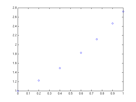
and you want to interpolate this data on a fine grid between x=0 and x=1 using piecewise cubic Hermite interpolation. One way of doing this in MATLAB is to use the interp1 function as follows
tic
t=0:0.00005:1;
y1 = interp1(x,y,t,'pchip');
toc
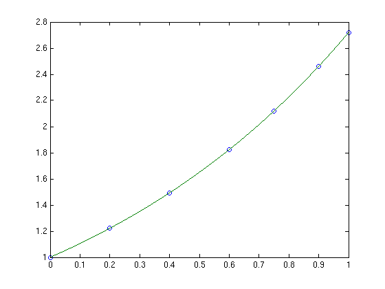
The tic and toc statements are there simply to provide timing information and on my system the above code took 0.503 seconds. We can do exactly the same calculation using the NAG toolbox for MATLAB:
tic
[d,ifail] = e01be(x,y);
[y2, ifail] = e01bf(x,y,d,t);
toc
which took 0.054958 seconds on my system making it around 9 times faster than the pure MATLAB solution – not bad at all for such a tiny amount of work. Of course y1 and y2 are identical as the following call to norm demonstrates
norm(y1-y2)
ans =
      0
Of course the real code contained a lot more than just a call to interp1 but using the above technique decreased the run time of the user’s application from 1 hour 10 minutes down to only 26 minutes.
Thanks to the NAG technical support team for their assistance with this particular problem and to the postgraduate student who came up with the idea in the first place.