
Archive for the ‘programming’ Category
So, you’re the proud owner of a new license for MATLAB’s parallel computing toolbox (PCT) and you are wondering how to get some bang for your buck as quickly as possible. Sure, you are going to learn about constructs such as parfor and spmd but that takes time and effort. Wouldn’t it be nice if you could speed up some of your MATLAB code simply by saying ‘Turn parallelisation on’?
It turns out that The Mathworks have been adding support for their parallel computing toolbox all over the place and all you have to do is switch it on (Assuming that you actually have the parallel computing toolbox of course). For example say you had the following call to fmincon (part of the optimisation toolbox) in your code
[x, fval] = fmincon(@objfun, x0, [], [], [], [], [], [], @confun,opts)
To turn on parallelisation across 2 cores just do
matlabpool 2;
opts = optimset('fmincon');
opts = optimset('UseParallel','always');
[x, fval] = fmincon(@objfun, x0, [], [], [], [], [], [], @confun,opts);
That wasn’t so hard was it? The speedup (if any) completely depends upon your particular optimization problem.
Why isn’t parallelisation turned on by default?
The next question that might occur to you is ‘Why doesn’t The Mathworks just turn parallelisation on by default?’ After all, although the above modification is straightforward, it does require you to know that this particular function supports parallel execution via the PCT. If you didn’t think to check then your code would be doomed to serial execution forever.
The simple answer to this question is ‘Sometimes the parallel version is slower‘. Take this serial code for example.
objfun = @(x)exp(x(1))*(4*x(1)^2+2*x(2)^2+4*x(1)*x(2)+2*x(2)+1);
confun = @(x) deal( [1.5+x(1)*x(2)-x(1)-x(2); -x(1)*x(2)-10], [] );
tic;
[x, fval] = fmincon(objfun, x0, [], [], [], [], [], [], confun);
toc
On the machine I am currently sat at (quad core running MATLAB 2011a on Linux) this typically takes around 0.032 seconds to solve. With a problem that trivial my gut feeling is that we are not going to get much out of switching to parallel mode.
objfun = @(x)exp(x(1))*(4*x(1)^2+2*x(2)^2+4*x(1)*x(2)+2*x(2)+1);
confun = @(x) deal( [1.5+x(1)*x(2)-x(1)-x(2); -x(1)*x(2)-10],[] );

%only do this next line once.  It opens two MATLAB workers
matlabpool 2;

opts = optimset('fmincon');
opts = optimset('UseParallel','always');

tic;
[x, fval] = fmincon(objfun, x0, [], [], [], [], [], [], confun,opts);
toc
Sure enough, this increases execution time dramatically to an average of 0.23 seconds on my machine. There is always a computational overhead that needs paying when you go parallel and if your problem is too trivial then this overhead costs more than the calculation itself.
So which functions support the Parallel Computing Toolbox?
I wanted a web-page that listed all functions that gain benefit from the Parallel Computing Toolbox but couldn’t find one. I found some documentation on specific toolboxes such as Parallel Statistics but nothing that covered all of MATLAB in one place. Here is my attempt at producing such a document. Feel free to contact me if I have missed anything out.
This covers MATLAB 2011b and is almost certainly incomplete. I’ve only covered toolboxes that I have access to and so some are missing. Please contact me if you have any extra information.
Bioinformatics Toolbox
Global Optimisation
- Various solvers use the PCT. See this part of the MATLAB documentation for details.
Image Processing
- blockproc
- Note that many Image Processing functions run in parallel even without the parallel computing toolbox. See my article Which MATLAB functions are Multicore Aware?
Optimisation Toolbox
Simulink
- Running parallel simulations
- You can increase the speed of diagram updates for models containing large model reference hierarchies by building referenced models that are configured in Accelerator mode in parallel whenever conditions allow. This is covered in the documentation.
Statistics Toolbox
- bootstrp
- bootci
- cordexch
- candexch
- crossval
- dcovary
- daugment
- growTrees
- jackknife
- lasso
- nnmf
- plsregress
- rowexch
- sequentialfs
- TreeBagger
Other articles about parallel computing in MATLAB from WalkingRandomly
- Which MATLAB functions are multicore aware? There are a ton of functions in MATLAB that take advantage of parallel processors automatically. No Parallel Computing Toolbox necessary.
- Parallel MATLAB with OpenMP mex files Want to parallelize your own functions without purchasing the PCT? Not afraid to get your hands dirty with C? Perhaps this option is for you.
- MATLAB GPU/CUDA Experiences and tutorials on my laptop – A series of articles where I look a GPU computing with CUDA on MATLAB
This is part 1 of an ongoing series of articles about MATLAB programming for GPUs using the Parallel Computing Toolbox. The introduction and index to the series is at https://www.walkingrandomly.com/?p=3730.
Have you ever needed to take the sine of 100 million random numbers? Me either, but such an operation gives us an excuse to look at the basic concepts of GPU computing with MATLAB and get an idea of the timings we can expect for simple elementwise calculations.
Taking the sine of 100 million numbers on the CPU
Let’s forget about GPUs for a second and look at how this would be done on the CPU using MATLAB. First, I create 100 million random numbers over a range from 0 to 10*pi and store them in the variable cpu_x;
cpu_x = rand(1,100000000)*10*pi;
Now I take the sine of all 100 million elements of cpu_x using a single command.
cpu_y = sin(cpu_x)
I have to confess that I find the above command very cool. Not only are we looping over a massive array using just a single line of code but MATLAB will also be performing the operation in parallel. So, if you have a multicore machine (and pretty much everyone does these days) then the above command will make good use of many of those cores. Furthermore, this kind of parallelisation is built into the core of MATLAB….no parallel computing toolbox necessary. As an aside, if you’d like to see a list of functions that automatically run in parallel on the CPU then check out my blog post on the issue.
So, how quickly does my 4 core laptop get through this 100 million element array? We can find out using the MATLAB functions tic and toc. I ran it three times on my laptop and got the following
>> tic;cpu_y = sin(cpu_x);toc
Elapsed time is 0.833626 seconds.
>> tic;cpu_y = sin(cpu_x);toc
Elapsed time is 0.899769 seconds.
>> tic;cpu_y = sin(cpu_x);toc
Elapsed time is 0.916969 seconds.
So the first thing you’ll notice is that the timings vary and I’m not going to go into the reasons why here. What I am going to say is that because of this variation it makes sense to time the calculation a number of times (20 say) and take an average. Let’s do that
sintimes=zeros(1,20);
for i=1:20;tic;cpu_y = sin(cpu_x);sintimes(i)=toc;end
average_time = sum(sintimes)/20

average_time =
    0.8011
So, on average, it takes my quad core laptop just over 0.8 seconds to take the sine of 100 million elements using the CPU. A couple of points:
- I note that this time is smaller than any of the three test times I did before running the loop and I’m not really sure why. I’m guessing that it takes my CPU a short while to decide that it’s got a lot of work to do and ramp up to full speed but further insights are welcomed.
- While staring at the CPU monitor I noticed that the above calculation never used more than 50% of the available virtual cores. It’s using all 4 of my physical CPU cores but perhaps if it took advantage of hyperthreading I’d get even better performance? Changing OMP_NUM_THREADS to 8 before launching MATLAB did nothing to change this.
Taking the sine of 100 million numbers on the GPU
Just like before, we start off by using the CPU to generate the 100 million random numbers1
cpu_x = rand(1,100000000)*10*pi;
The first thing you need to know about GPUs is that they have their own memory that is completely separate from main memory. So, the GPU doesn’t know anything about the array created above. Before our GPU can get to work on our data we have to transfer it from main memory to GPU memory and we acheive this using the gpuArray command.
gpu_x = gpuArray(cpu_x); %this moves our data to the GPU
Once the GPU can see all our data we can apply the sine function to it very easily.
gpu_y = sin(gpu_x)
Finally, we transfer the results back to main memory.
cpu_y = gather(gpu_y)
If, like many of the GPU articles you see in the literature, you don’t want to include transfer times between GPU and host then you time the calculation like this:
tic
gpu_y = sin(gpu_x);
toc
Just like the CPU version, I repeated this calculation several times and took an average. The result was 0.3008 seconds giving a speedup of 2.75 times compared to the CPU version.
If, however, you include the time taken to transfer the input data to the GPU and the results back to the CPU then you need to time as follows
tic
gpu_x = gpuArray(cpu_x);
gpu_y = sin(gpu_x);
cpu_y = gather(gpu_y)
toc
On my system this takes 1.0159 seconds on average– longer than it takes to simply do the whole thing on the CPU. So, for this particular calculation, transfer times between host and GPU swamp the benefits gained by all of those CUDA cores.
Benchmark code
I took the ideas above and wrote a simple benchmark program called sine_test. The way you call it is as follows
[cpu,gpu_notransfer,gpu_withtransfer] = sin_test(numrepeats,num_elements]
For example, if you wanted to run the benchmarks 20 times on a 1 million element array and return the average times then you just do
>> [cpu,gpu_notransfer,gpu_withtransfer] = sine_test(20,1e6)
cpu =
    0.0085
gpu_notransfer =
    0.0022
gpu_withtransfer =
    0.0116
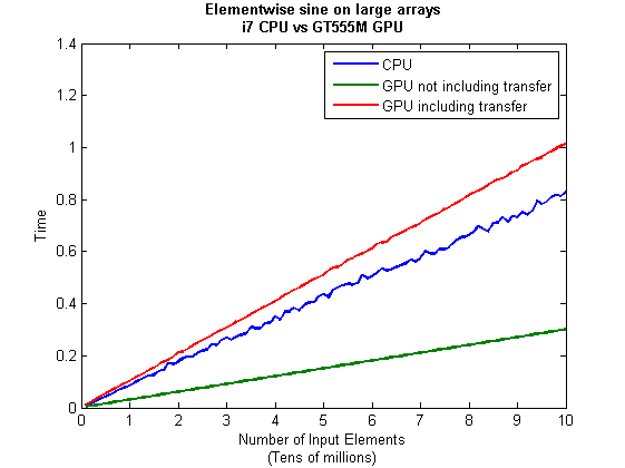
I then ran this on my laptop for array sizes ranging from 1 million to 100 million and used the results to plot the graph below.
But I wanna write a ‘GPUs are awesome’ paper
So far in this little story things are not looking so hot for the GPU and yet all of the ‘GPUs are awesome’ papers you’ve ever read seem to disagree with me entirely. What on earth is going on? Well, lets take the advice given by csgillespie.wordpress.com and turn it on its head. How do we get awesome speedup figures from the above benchmarks to help us pump out a ‘GPUs are awesome paper’?
0. Don’t consider transfer times between CPU and GPU.
We’ve already seen that this can ruin performance so let’s not do it shall we? As long as we explicitly say that we are not including transfer times then we are covered.
1. Use a singlethreaded CPU.
Many papers in the literature compare the GPU version with a single-threaded CPU version and yet I’ve been using all 4 cores of my processor. Silly me…let’s fix that by running MATLAB in single threaded mode by launching it with the command
matlab -singleCompThread
Now when I run the benchmark for 100 million elements I get the following times
>> [cpu,gpu_no,gpu_with] = sine_test(10,1e8)
cpu =
    2.8875
gpu_no =
    0.3016
gpu_with =
    1.0205
Now we’re talking! I can now claim that my GPU version is over 9 times faster than the CPU version.
2. Use an old CPU.
My laptop has got one of those new-fangled sandy-bridge i7 processors…one of the best classes of CPU you can get for a laptop. If, however, I was doing these tests at work then I guess I’d be using a GPU mounted in my university Desktop machine. Obviously I would compare the GPU version of my program with the CPU in the Desktop….an Intel Core 2 Quad Q9650. Heck its running at 3Ghz which is more Ghz than my laptop so to the casual observer (or a phb) it would look like I was using a more beefed up processor in order to make my comparison fairer.
So, I ran the CPU benchmark on that (in singleCompThread mode obviously) and got 4.009 seconds…noticeably slower than my laptop. Awesome…I am definitely going to use that figure!
I know what you’re thinking…Mike’s being a fool for the sake of it but csgillespie.wordpress.com puts it like this ‘Since a GPU has (usually) been bought specifically for the purpose of the article, the CPU can be a few years older.’ So, some of those ‘GPU are awesome’ articles will be accidentally misleading us in exactly this manner.
3. Work in single precision.
Yeah I know that you like working with double precision arithmetic but that slows GPUs down. So, let’s switch to single precision. Just argue in your paper that single precision is OK for this particular calculation and we’ll be set. To change the benchmarking code all you need to do is change every instance of
rand(1,num_elems)*10*pi;
to
rand(1,num_elems,'single')*10*pi;
Since we are reputable researchers we will, of course, modify both the CPU and GPU versions to work in single precision. Timings are below
- Desktop at work (single thread, single precision): 3.49 seconds
- Laptop GPU (single precision, not including transfer): 0.122 seconds
OK, so switching to single precision made the CPU version a bit faster but it’s more than doubled GPU performance. We can now say that the GPU version is over 28 times faster than the CPU version. Now we have ourselves a bone-fide ‘GPUs are awesome’ paper.
4. Use the best GPU we can find
So far I have been comparing the CPU against the relatively lowly GPU in my laptop. Obviously, however, if I were to do this for real then I’d get a top of the range Tesla. It turns out that I know someone who has a Tesla C2050 and so we ran the single precision benchmark on that. The result was astonishing…0.0295 seconds for 100 million numbers not including transfer times. The double precision performance for the same calculation on the C2050 was 0.0524 seonds.
5. Write the abstract for our ‘GPUs are awesome’ paper
We took an Nvidia Tesla C2050 GPU and mounted it in a machine containing an Intel Quad Core CPU running at 3Ghz. We developed a program that performs element-wise trigonometry on arrays of up to 100 million single precision random numbers using both the CPU and the GPU. The GPU version of our code ran up to 118 times faster than the CPU version. GPUs are awesome!
Results from different CPUs and GPUs. Double precision, multi-threaded
I ran the sine_test benchmark on several different systems for 100 million elements. The CPU was set to be multi-threaded and double precision was used throughout.
sine_test(10,1e8)
GPUs
- Tesla C2050, Linux, 2011a – 0.7487 seconds including transfers, 0.0524 seconds excluding transfers.
- GT 555M – 144 CUDA Cores, 3Gb RAM, Windows 7, 2011a (My laptop’s GPU) -1.0205 seconds including transfers, 0.3016 seconds excluding transfers
CPUs
- Intel Core i7-880 @3.07Ghz, Linux, 2011a – 0.659 seconds
- Intel Core i7-2630QM, Windows 7, 2011a (My laptop’s CPU) – 0.801 seconds
- Intel Core 2 Quad Q9650 @ 3.00GHz, Linux – 0.958 seconds
Conclusions
- MATLAB’s new GPU functions are very easy to use! No need to learn low-level CUDA programming.
- It’s very easy to massage CPU vs GPU numbers to look impressive. Read those ‘GPUs are awesome’ papers with care!
- In real life you have to consider data transfer times between GPU and CPU since these can dominate overall wall clock time with simple calculations such as those considered here. The more work you can do on the GPU, the better.
- My laptop’s GPU is nowhere near as good as I would have liked it to be. Almost 6 times slower than a Tesla C2050 (excluding data transfer) for elementwise double precision calculations. Data transfer times seem to about the same though.
Next time
In the next article in the series I’ll look at an element-wise calculation that really is worth doing on the GPU – even using the wimpy GPU in my laptop – and introduce the MATLAB function arrayfun.
Footnote
1 – MATLAB 2011a can’t create random numbers directly on the GPU. I have no doubt that we’ll be able to do this in future versions of MATLAB which will change the nature of this particular calculation somewhat. Then it will make sense to include the random number generation in the overall benchmark; transfer times to the GPU will be non-existant. In general, however, we’ll still come across plenty of situations where we’ll have a huge array in main memory that needs to be transferred to the GPU for further processing so what we learn here will not be wasted.
Hardware / Software used for the majority of this article
- Laptop model: Dell XPS L702X
- CPU: Intel Core i7-2630QM @2Ghz software overclockable to 2.9Ghz. 4 physical cores but total 8 virtual cores due to Hyperthreading.
- GPU: GeForce GT 555M with 144 CUDA Cores. Graphics clock: 590Mhz. Processor Clock:1180 Mhz. 3072 Mb DDR3 Memeory
- RAM: 8 Gb
- OS: Windows 7 Home Premium 64 bit. I’m not using Linux because of the lack of official support for Optimus.
- MATLAB: 2011a with the parallel computing toolbox
Other GPU articles at Walking Randomly
- GPU Support in Mathematica, Maple, MATLAB and Maple Prime – See the various options available
- Insert new laptop to continue – My first attempt at using the GPU functionality in MATLAB
- NVIDIA lets down Linux laptop users – and how an open source project saves the day
Thanks to various people at The Mathworks for some useful discussions, advice and tutorials while creating this series of articles.
These days it seems that you can’t talk about scientific computing for more than 5 minutes without somone bringing up the topic of Graphics Processing Units (GPUs). Originally designed to make computer games look pretty, GPUs are massively parallel processors that promise to revolutionise the way we compute.
A brief glance at the specification of a typical laptop suggests why GPUs are the new hotness in numerical computing. Take my new one for instance, a Dell XPS L702X, which comes with a Quad-Core Intel i7 Sandybridge processor running at up to 2.9Ghz and an NVidia GT 555M with a whopping 144 CUDA cores. If you went back in time a few years and told a younger version of me that I’d soon own a 148 core laptop then young Mike would be stunned. He’d also be wondering ‘What’s the catch?’
Of course the main catch is that all processor cores are not created equally. Those 144 cores in my GPU are, individually, rather wimpy when compared to the ones in the Intel CPU. It’s the sheer quantity of them that makes the difference. The question at the forefront of my mind when I received my shiny new laptop was ‘Just how much of a difference?’
Now I’ve seen lots of articles that compare CPUs with GPUs and the GPUs always win…..by a lot! Dig down into the meat of these articles, however, and it turns out that things are not as simple as they seem. Roughly speaking, the abstract of some them could be summed up as ‘We took a serial algorithm written by a chimpanzee for an old, outdated CPU and spent 6 months parallelising and fine tuning it for a top of the line GPU. Our GPU version is up to 150 times faster!‘
Well it would be wouldn’t it?! In other news, Lewis Hamilton can drive his F1 supercar around Silverstone faster than my dad can in his clapped out 12 year old van! These articles are so prevalent that csgillespie.wordpress.com recently published an excellent article that summarised everything you should consider when evaluating them. What you do is take the claimed speed-up, apply a set of common sense questions and thus determine a realistic speedup. That factor of 150 can end up more like a factor of 8 once you think about it the right way.
That’s not to say that GPUs aren’t powerful or useful…it’s just that maybe they’ve been hyped up a bit too much!
So anyway, back to my laptop. It doesn’t have a top of the range GPU custom built for scientific computing, instead it has what Notebookcheck.net refers to as a fast middle class graphics card for laptops. It’s got all of the required bits though….144 cores and CUDA compute level 2.1 so surely it can whip the built in CPU even if it’s just by a little bit?
I decided to find out with a few randomly chosen tests. I wasn’t aiming for the kind of rigor that would lead to a peer reviewed journal but I did want to follow some basic rules at least
- I will only choose algorithms that have been optimised and parallelised for both the CPU and the GPU.
- I will release the source code of the tests so that they can be critised and repeated by others.
- I’ll do the whole thing in MATLAB using the new GPU functionality in the parallel computing toolbox. So, to repeat my calculations all you need to do is copy and paste some code. Using MATLAB also ensures that I’m using good quality code for both CPU and GPU.
The articles
This is the introduction to a set of articles about GPU computing on MATLAB using the parallel computing toolbox. Links to the rest of them are below and more will be added in the future.
- Elementwise operations on the GPU #1 – Basic commands using the PCT and how to write a ‘GPUs are awesome’ paper; no matter what results you get!
- Elementwise operations on the GPU #2 – A slightly more involved example showing a useful speed-up compared to the CPU. An introduction to MATLAB’s arrayfun
- Optimising a correlated asset calculation on MATLAB #1: Vectorisation on the CPU – A detailed look at a port from CPU MATLAB code to GPU MATLAB code.
- Optimising a correlated asset calculation on MATLAB #2: Using the GPU via the PCT – A detailed look at a port from CPU MATLAB code to GPU MATLAB code.
- Optimising a correlated asset calculation on MATLAB #3: Using the GPU via Jacket – A detailed look at a port from CPU MATLAB code to GPU MATLAB code.
External links of interest to MATLABers with an interest in GPUs
- The Parallel Computing Toolbox (PCT) – The Mathwork’s MATLAB add-on that gives you CUDA GPU support.
- Mike Gile’s MATLAB GPU Blog – from the University of Oxford
- Accelereyes – Developers of ‘Jacket’, an alternative to the parallel computing toolbox.
- A Mandelbrot Set on the GPU – Using the parallel computing toolbox to make pretty pictures…FAST!
- GP-you.org – A free CUDA-based GPU toolbox for MATLAB
- Matlab, CUDA and Me – Stu Blair gives various examples of calling CUDA kernels directly from MATLAB
Over at Sol Lederman’s fantastic new blog, Playing with Mathematica, he shared some code that produced the following figure.

Here’s Sol’s code with an AbsoluteTiming command thrown in.
f[x_, y_] := Module[{},
  If[
   Sin[Min[x*Sin[y], y*Sin[x]]] >
    Cos[Max[x*Cos[y],
       y*Cos[x]]] + (((2 (x - y)^2 + (x + y - 6)^2)/40)^3)/
      6400000 + (12 - x - y)/30, 1, 0]
  ]

 AbsoluteTiming[
\[Delta] = 0.02;
range = 11;
xyPoints = Table[{x, y}, {y, 0, range, \[Delta]}, {x, 0, range, \[Delta]}];
image = Map[f @@ # &, xyPoints, {2}];
]
Rotate[ArrayPlot[image, ColorRules -> {0 -> White, 1 -> Black}], 135 Degree]
This took 8.02 seconds on the laptop I am currently working on (Windows 7 AMD Phenom II N620 Dual core at 2.8Ghz). Note that I am only measuring how long the calculation itself took and am ignoring the time taken to render the image and define the function.
Compiled functions make Mathematica code go faster
Mathematica has a Compile function which does exactly what you’d expect…it produces a compiled version of the function you give it (if it can!). Sol’s function gave it no problems at all.
f = Compile[{{x, _Real}, {y, _Real}}, If[
    Sin[Min[x*Sin[y], y*Sin[x]]] >
     Cos[Max[x*Cos[y],
        y*Cos[x]]] + (((2 (x - y)^2 + (x + y - 6)^2)/40)^3)/
       6400000 + (12 - x - y)/30, 1, 0]
   ];

AbsoluteTiming[
 \[Delta] = 0.02;
 range = 11;
 xyPoints =
  Table[{x, y}, {y, 0, range, \[Delta]}, {x, 0, range, \[Delta]}];
 image = Map[f @@ # &, xyPoints, {2}];
 ]
Rotate[ArrayPlot[image, ColorRules -> {0 -> White, 1 -> Black}],
 135 Degree]
This simple change takes computation time down from 8.02 seconds to 1.23 seconds which is a 6.5 times speed up for hardly any extra coding work. Not too shabby!
Switch to C code to get it even faster
I’m not done yet though! By default the Compile command produces code for the so-called Mathematica Virtual Machine but recent versions of Mathematica allow us to go even further.
Install Visual Studio Express 2010 (and the Windows 7.1 SDK if you are running 64bit Windows) and you can ask Mathematica to convert the function to low level C code, compile it and produce a function object linked to the resulting compiled code. Sounds complicated but is a snap to actually do. Just add
CompilationTarget -> "C"
to the Compile command.
f = Compile[{{x, _Real}, {y, _Real}},
   If[Sin[Min[x*Sin[y], y*Sin[x]]] >
     Cos[Max[x*Cos[y],
        y*Cos[x]]] + (((2 (x - y)^2 + (x + y - 6)^2)/40)^3)/
       6400000 + (12 - x - y)/30, 1, 0]
   , CompilationTarget -> "C"
   ];

AbsoluteTiming[\[Delta] = 0.02;
 range = 11;
 xyPoints =
  Table[{x, y}, {y, 0, range, \[Delta]}, {x, 0, range, \[Delta]}];
 image = Map[f @@ # &, xyPoints, {2}];]
Rotate[ArrayPlot[image, ColorRules -> {0 -> White, 1 -> Black}],
 135 Degree]
On my machine this takes calculation time down to 0.89 seconds which is 9 times faster than the original.
Making the compiled function listable
The current compiled function takes just one x,y pair and returns a result.
In[8]:= f[1, 2]

Out[8]= 1
It can’t directly accept a list of x values and a list of y values. For example for the two points (1,2) and (10,20) I’d like to be able to do f[{1, 10}, {2, 20}] and get the results {1,1}. However what I end up with is an error
f[{1, 10}, {2, 20}]

CompiledFunction::cfsa: Argument {1,10} at position 1 should be a machine-size real number. >>
To fix this I need to make my compiled function listable which is as easy as adding
RuntimeAttributes -> {Listable}
to the function definition.
f = Compile[{{x, _Real}, {y, _Real}},
   If[Sin[Min[x*Sin[y], y*Sin[x]]] >
     Cos[Max[x*Cos[y],
        y*Cos[x]]] + (((2 (x - y)^2 + (x + y - 6)^2)/40)^3)/
       6400000 + (12 - x - y)/30, 1, 0]
   , CompilationTarget -> "C", RuntimeAttributes -> {Listable}
   ];
So now I can pass the entire array to this compiled function at once. No need for Map.
AbsoluteTiming[
 \[Delta] = 0.02;
 range = 11;
 xpoints = Table[x, {x, 0, range, \[Delta]}, {y, 0, range, \[Delta]}];
 ypoints = Table[y, {x, 0, range, \[Delta]}, {y, 0, range, \[Delta]}];
 image = f[xpoints, ypoints];
 ]
Rotate[ArrayPlot[image, ColorRules -> {0 -> White, 1 -> Black}],
 135 Degree]
On my machine this gets calculation time down to 0.28 seconds, a whopping 28.5 times faster than the original. Rendering time is becoming much more of an issue than calculation time in fact!
Parallel anyone?
Simply by adding
Parallelization -> True
to the Compile command I can parallelise the code using threads. Since I have a dual core machine, this might be a good thing to do. Let’s take a look
f = Compile[{{x, _Real}, {y, _Real}},
   If[
    Sin[Min[x*Sin[y], y*Sin[x]]] >
     Cos[Max[x*Cos[y],
        y*Cos[x]]] + (((2 (x - y)^2 + (x + y - 6)^2)/40)^3)/
       6400000 + (12 - x - y)/30, 1, 0]
   , RuntimeAttributes -> {Listable}, CompilationTarget -> "C",
   Parallelization -> True];

AbsoluteTiming[
 \[Delta] = 0.02;
 range = 11;
 xpoints = Table[x, {x, 0, range, \[Delta]}, {y, 0, range, \[Delta]}];
 ypoints = Table[y, {x, 0, range, \[Delta]}, {y, 0, range, \[Delta]}];
 image = f[xpoints, ypoints];
 ]
Rotate[ArrayPlot[image, ColorRules -> {0 -> White, 1 -> Black}],
 135 Degree]
The first time I ran this it was SLOWER than the non-threaded version coming in at 0.33 seconds. Subsequent runs varied and occasionally got as low as 0.244 seconds which is only a few hundredths of a second faster than the original.
If I make the problem bigger, however, by decreasing the size of Delta then we start to see the benefit of parallelisation.
AbsoluteTiming[
 \[Delta] = 0.01;
 range = 11;
 xpoints = Table[x, {x, 0, range, \[Delta]}, {y, 0, range, \[Delta]}];
 ypoints = Table[y, {x, 0, range, \[Delta]}, {y, 0, range, \[Delta]}];
 image = f[xpoints, ypoints];
 ]
Rotate[ArrayPlot[image, ColorRules -> {0 -> White, 1 -> Black}],
 135 Degree]
The above calculation (sans rendering) took 0.988 seconds using a parallelised version of f and 1.24 seconds using a serial version. Rendering took significantly longer! As a comparison lets put a Delta of 0.01 in the original code:
f[x_, y_] := Module[{},
  If[
   Sin[Min[x*Sin[y], y*Sin[x]]] >
    Cos[Max[x*Cos[y],
       y*Cos[x]]] + (((2 (x - y)^2 + (x + y - 6)^2)/40)^3)/
      6400000 + (12 - x - y)/30, 1, 0]
  ]

 AbsoluteTiming[
\[Delta] = 0.01;
range = 11;
xyPoints = Table[{x, y}, {y, 0, range, \[Delta]}, {x, 0, range, \[Delta]}];
image = Map[f @@ # &, xyPoints, {2}];
]
Rotate[ArrayPlot[image, ColorRules -> {0 -> White, 1 -> Black}], 135 Degree]
The calculation time (again, ignoring rendering time) took 32.56 seconds and so our C-compiled, parallel version is almost 33 times faster!
Summary
- The Compile function can make your code run significantly faster by compiling it for the Mathematica Virtual Machine (MVM). Note that not every function is suitable for compilation.
- If you have a C-compiler installed on your machine then you can switch from the MVM to compiled C-code using a single option statement. The resulting code is even faster
- Making your functions listable can increase performance.
- Parallelising your compiled function is easy and can lead to even more speed but only if your problem is of a suitable size.
- Sol Lederman has a very cool Mathematica blog – check it out! The code that inspired this blog post originated there.
One part of my job that I really enjoy is the optimisation of researcher’s code. Typically, the code comes to me in a language such as MATLAB or Mathematica and may take anywhere from a couple of hours to several weeks to run. I’ve had some nice successes recently in areas as diverse as finance, computer science, applied math and chemical engineering among others. The size of the speed-up can vary from 10% right up to 5000% (yes, 50 times faster!) and that’s before I break out the big guns such as Manchester’s Condor pool or turn the code over to our HPC specialists for some SERIOUS (yet more time consuming in terms of developer time) optimisations.
Reporting these speed-ups to colleagues (along with the techniques I used) gets various responses such as ‘Well, they shouldn’t do time-consuming computing using high level languages. They should rewrite the whole thing in Fortran’ or words to that effect. I disagree!
In my opinion, high level programming languages such as Mathematica, MATLAB and Python have democratised scientific programming. Now, almost anyone who can think logically can turn their scientific ideas into working code. I’ve seen people who have had no formal programming training at all whip up models, get results and move on with their research. Let’s be clear here – It’s results that matter not how you coded them.
It comes down to this. CPU time is cheap. Very cheap. Human time, particularly specialised human time, is expensive.
Here’s an example: Earlier this year I was working with a biologist who had put together some MATLAB code to analyse her data. She had written the code in less than a day and it gave the correct results but it ran too slowly for her tastes. Her sole programming experience came from reading the MATLAB manual and yet she could cook up useful code in next to no time. Sure, it was slow and (to my eyes) badly written but give the gal a break…she’s a professional biologist and not a professional programmer. Her programming is a lot better than my biology!
In less than two hours I gave her a crash course in MATLAB code optimisation; how to use the profiler, vectorisation and so on. We identified the hotspot in the code and, between us, recoded it so that it was an order of magnitude faster. This was more than fast enough for her needs, she could now analyse data significantly faster than she could collect it. I realised that I could make it even faster by using parallelised mex functions but it would probably take a few more hours work. She declined my offer…the code was fast enough.
In my opinion, this is an optimal use of resources. I spend my days obsessing about mathematical software and she spends her days obsessing about experimental biology. She doesn’t need a formal course in how to write uber-efficient code because her code runs as fast as she needs it to (with a little help from her friends). The solution we eventually reached might not be the most CPU-efficient one but it is a good trade off between CPU-efficient and developer-efficient.
It was easy…trivial even..for someone like me to take her inefficient code and turn it into something that was efficient enough. However, the whole endeavour relied on her producing working code in the first place. Say high-level languages such as MATLAB didn’t exist….then her only options would be to hire a professional programmer (cash expensive) or spend a load of time learning how to code in a low level language such as Fortran or C (time expensive).
Also, because she is a beginner programmer, her C or Fortran code would almost certainly be crappy and one thing I am sure of is ‘Crappy MATLAB/Python/Mathematica/R code is a heck of a lot easier to debug and optimise than crappy C code.’ Segfault anyone?
MATLAB’s lsqcurvefit function is a very useful piece of code that will help you solve non-linear least squares curve fitting problems and it is used a lot by researchers at my workplace, The University of Manchester. As far as we are concerned it has two problems:
- lsqcurvefit is part of the Optimisation toolbox and, since we only have a limited number of licenses for that toolbox, the function is sometimes inaccessible. When we run out of licenses on campus users get the following error message
??? License checkout failed.
License Manager Error -4
Maximum number of users for Optimization_Toolbox reached.
Try again later.
To see a list of current users use the lmstat utility or contact your License Administrator.
- lsqcurvefit is written as an .m file and so isn’t as fast as it could be.
One solution to these problems is to switch to the NAG Toolbox for MATLAB. Since we have a full site license for this product, we never run out of licenses and, since it is written in compiled Fortran, it is sometimes a lot faster than MATLAB itself. However, the current version of the NAG Toolbox (Mark 22 at the time of writing) isn’t without its issues either:
- There is no direct equivalent to lsqcurvefit in the NAG toolbox. You have to use NAG’s equivalent of lsqnonlin instead (which NAG call e04fy)
- The current version of the NAG Toolbox, Mark 22, doesn’t support function handles.
- The NAG toolbox requires the use of the datatypes int32 and int64 depending on the architecture of your machine. The practical upshot of this is that your MATLAB code is suddenly a lot less portable. If you develop on a 64 bit machine then it will need modifying to run on a 32 bit machine and vice-versa.
While working on optimising someone’s code a few months ago I put together a couple of .m files in an attempt to address these issues. My intent was to improve the functionality of these files and eventually publish them but I never seemed to find the time. However, they have turned out to be a minor hit and I’ve sent them out to researcher after researcher with the caveat “These are a first draft, I need to tidy them up sometime” only to get the reply “Thanks for that, I no longer have any license problems and my code is executing more quickly.” They may be simple but it seems that they are useful.
So, until I find the time to add more functionality, here are my little wrappers that allow you to do non linear least squares fitting using the NAG Toolbox for MATLAB. They are about as minimal as you can get but they work and have proven to be useful time and time again. They also solve all 3 of the NAG issues mentioned above.
To use them just put them both somewhere on your MATLAB path. The syntax is identical to lsqcurvefit but this first version of my wrapper doesn’t do anything more complicated than the following
MATLAB:
[x,resnorm] = lsqcurvefit(@myfun,x0,xdata,ydata);
NAG with my wrapper:
[x,resnorm] = nag_lsqcurvefit(@myfun,x0,xdata,ydata);
I may add extra functionality in the future but it depends upon demand.
Performance
Let’s look at the example given on the MATLAB help page for lsqcurvefit and compare it to the NAG version. First create a file called myfun.m as follows
function F = myfun(x,xdata)
F = x(1)*exp(x(2)*xdata);
Now create the data and call the MATLAB fitting function
% Assume you determined xdata and ydata experimentally
xdata = [0.9 1.5 13.8 19.8 24.1 28.2 35.2 60.3 74.6 81.3];
ydata = [455.2 428.6 124.1 67.3 43.2 28.1 13.1 -0.4 -1.3 -1.5];
x0 = [100; -1] % Starting guess
[x,resnorm] = lsqcurvefit(@myfun,x0,xdata,ydata);
On my system I get the following timing for MATLAB (typical over around 10 runs)
tic;[x,resnorm] = lsqcurvefit(@myfun,x0,xdata,ydata); toc
Elapsed time is 0.075685 seconds.
with the following results
x =
   1.0e+02 *
   4.988308584891165
  -0.001012568612537
>> resnorm
resnorm =
   9.504886892389219
and for NAG using my wrapper function I get the following timing (typical over around 10 runs)
tic;[x,resnorm] = nag_lsqcurvefit(@myfun,x0,xdata,ydata); toc
Elapsed time is 0.008163 seconds.
So, for this example, NAG is around 9 times faster! The results agree with MATLAB to several decimal places
x =
   1.0e+02 *
   4.988308605396028
  -0.001012568632465
>> resnorm
resnorm =
   9.504886892366873
In the real world I find that the relative timings vary enormously and have seen speed-ups that range from a factor of 14 down to none at all. Whenever I am optimisng MATLAB code and see a lsqcurvefit function I always give the NAG version a quick try and am often impressed with the results.
My system specs if you want to compare results: 64bit Linux on a Intel Core 2 Quad Q9650 @ 3.00GHz running MATLAB 2010b and NAG Toolbox version MBL6A22DJL
More articles about NAG
Last month I published an article that included an interactive mathematical demonstration powered by Wolfram’s new CDF (Computable Document Format) player. These demonstrations work on many modern web-browsers including Internet Explorer 8 and Firefox 3.6. So, how do you go about adding them to your own websites?
What you need
- Mathematica 8.0.1 or above to create demonstrations. Viewers of your demonstration only need the free CDF player for their platform.
- A modern browser such as Internet Explorer 8, Firefox 3.6 or Safari 5.
- Basic knowledge of HTML, uploading files to a webserver etc. If you maintain a blog or similar then you almost certainly know enough
Our aim is the following, very simple, interactive demonstration.
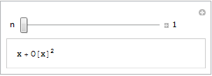
If all you see is a static image then you do not have the CDF player or Mathematica 8 correctly installed. Alternatively, you are using an unsupported platform such as Linux, iOS or Android.
Step 1 – Create the .cdf file
Fire up Mathematica, type in and evaluate the following code. You should get an applet similar to the one above.
Manipulate[
 Series[Sin[x], {x, 0, n}]
 , {n, 1, 10, 1, Appearance -> "Labeled"}
 ]
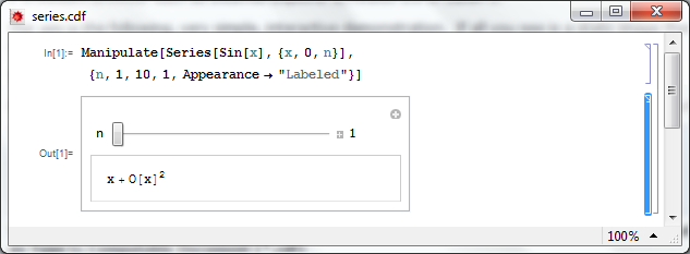
Save it as a .cdf file called series.cdf by clicking on File->Save as — Give it the File Name series.cdf and change the Save as Type to Computable Document (*.cdf)

Step 2 – Get a static screenshot
Not everyone is going to have either Mathematica 8 or the free CDF player installed when they visit your website so we need to give them something to look at. So, lets give them a static image of the Manipulate applet. As a bonus, this will act as a place holder for the interactive version for those who do have the requisite software.
Open series.cdf in Mathematica and left click on the bracket surrounding the manipulate (see below). Click on Cell->Convert To->Bitmap. Then click on File->Save Selection As . Make sure you change .pdf to something more sensible such as .png
Don’t save your .cdf file at this point or it won’t be interactive. Re-evaluate the code again to get back your interactive Manipulate.
Here’s one I made earlier – series.png
Step 4 – Hide the source code
In this particular instance, I don’t want the user to see the source code. So, lets sort that out.
- Open series.cdf in Mathematica if you haven’t already and make sure that the Manipulate is evaluated.
- Left click on the inner cell bracket surrounding the Manipulate source code only and click on Cell->Cell Properties and un-tick Open
Step 5 – Hide the cell brackets
Those blue brackets at the far right of the Mathematica notebook are called the Cell brackets and I don’t want to see them on my web site as they make the applet look messy.
- Open series.cdf in Mathematica if you haven’t already
- Open the option inspector: Edit->Preferences->Advanced->Open Option Inspector
- Ensure Show option values is set to “series.cdf” and that they are sorted by category. Click on Apply.
- Click on Cell Options-> Display options and in the right hand pane set ShowCellBracket to False
- Click Apply
Before you save series.cdf ensure that the applet is interactive and not a static bitmap. If it isn’t interactive then click on Evaluation->Evaluate notebook to re-evaluate the (now hidden) source code. Also ensure that there is nothing but the applet anywhere else in the notebook.
Step 6 – Get interactive on your website
Upload series.png and series.cdf to your server. The next thing we need to do is get the static image into our webpage. Here’s what the HTML might look like
<img id="Series_applet" src="series.png" alt="Series demo" />
Obviously, you’ll need to put the full path to series.png on your server in this piece of code. The only thing that is different to the way you might usually use the img tag is that it includes an id; in this case it is Series_applet. We’ll make use of this later.
The magic happens thanks to a small javascript applet called the CDF javascript plugin. Version one is at http://www.wolfram.com/cdf-player/plugin/v1.0/cdfplugin.js and that’s the one I’ll be using here. Here’s the code which needs to be placed before the img tag in your HTML file.
<script src="http://www.wolfram.com/cdf-player/plugin/v1.0/cdfplugin.js"
type="text/javascript"></script><script type="text/javascript">// <![CDATA[
var cdf = new cdf_plugin();
cdf.addCDFObject("Series_applet", "series.cdf", 403,109);
// ]]></script>
The only line you’ll need to change if you use this for anything else is
cdf.addCDFObject("Series_applet", "series.cdf", 403,109);
where Series_applet is the id of the image we wish to replace and series.cdf is the cdf file we want to replace it with. The numbers 403,109 are the dimensions of the applet. These will not be the same as the .png file as the dimensions of the .cdf file are slightly larger. I used trial and error to determine what they should be as I haven’t come up with a better way yet (suggestions welcomed).
So that’s it for now. Hope this mini-tutorial was useful. Let me know if you upload any demonstrations to your own website or if you have any comments, questions or problems.
Update (6th June 2011)
Thanks to ‘Paul’ in the comments section, I have discovered that this mechanism won’t work for .cdf files that Wolfram deem are unsafe. According to Paul the definition of unsafe is as follows:
Dynamic content is considered unsafe if it:
- uses File operations
- uses interprocess communication via MathLink Mathematica Functions
- uses JLink or NETLink
- uses Low-Level Notebook Programming
- uses data as code by Converting between Expressions and Strings
- uses Namespace Management
- uses Options Management
- uses External Programs
A couple of weeks ago my friend and colleague, Ian Cottam, wrote a guest post here at Walking Randomly about his work on interfacing Dropbox with the high throughput computing software, Condor. Ian’s post was very well received and so he’s back; this time writing about a very different kind of project. Over to Ian.
Natural Scientists: their very big output files – and a tale of diffs by Ian Cottam
I’ve noticed that natural scientists (as opposed to computer scientists) often write, or use, programs that produce masses of output, usually just numbers. It might be the final results file or, often, some intermediate test results.
Am I being a little cynical in thinking that many users glance – ok, carefully check – a few of these thousands (millions?) of numbers and then delete the file? Let’s assume such files are really needed. A little automation is often added to the process by having a baseline file and running a program to show you the differences between it and your latest output (assuming wholesale changes are not the norm).
One of the popular difference programs is the Unix diff command . (I’ve been using it since the 1970s.) It popularised the idea of showing minimal differences between two text files (and, later, binary ones too). There are actually a few algorithms for doing minimal difference computation, and GNU diff, for example, uses a different one from the original Bell Labs version. They all have one thing in common: to achieve minimal difference computation the two files being compared must be read into main memory (aka RAM). Back in the 1970s, and on my then department’s PDP-11/40, this restricted the size of the files considerably; not that we noticed much as everything was 16bit and “small was beautiful”. GNU diff, on modern machines, can cope with very big files, but still chokes if your files, in aggregate, approach the gigabyte range.
(As a bit of an aside: a major contribution of all the GNU tools, over what we had been used to from the Unix pioneers at Bell Labs, was that they removed all arbitrary size restrictions; the most common and frustrating one being the length of text lines.)
Back to the 1970s again: Bell Labs did know that some files were too big to compare with diff , and they also shipped: diffh. The h stands for halfhearted. Diffh does not promise minimal differences, but can be very good for big files with occasional differences. It uses a pass over the files using a simple ‘sliding window’ heuristic approach (the other word that the h is sometimes said to stand for). You can still find an old version of diffh on the Internet. However, it ‘gives up’ rather easily and you may have to spend some time modifying it for, e.g., 64 bit ints and pointers, as well as for compiling with modern C compilers. Other tools exist that can compare enormous files, but they don’t produce readable output in diff’s pleasant format.
A few years back, when a user at the University of Manchester asked for help with the ‘diff – files too big/ out of memory’ problem, I wrote a modern version that I called idiffh (for Ian’s diffh). My ground rules were:
- Work on any text files on any operating system with a C compiler
- Have no limits on, e.g., line lengths or file size
- Never ‘give up’ if the going gets tough (i.e. when the files are very different)
You won’t find this with the GNU collection as they like to write code to the Unix interface and I like to write to the C standard I/O interface (see the first bullet point above).
An interesting implementation detail is that it uses random access to the files directly, relying on the operating system’s cache of file blocks to make this tolerably efficient. Waiting a minute or two to compare gigabyte sized files is usually acceptable.
As the comments in the code say, you can get some improvements by conditional compilation on Unix systems and especially on BSD Systems (including Apple Macs), but you can compile it straight, without such, on Windows and other platforms.
If you would like to try idffh out you can download it here.
My passions include mathematics, mathematical software and gadgets. So, I instantly fell in love with the LED Cube. The programming was done in C but MATLAB was used for some of the prototyping.
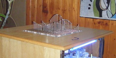
If you prefer something more physical then how about the MATLAB-controlled 3D function machine?
Perhaps you prefer a more retro, aural kind of a vibe? MATLAB-controlled carol singing dot-matrix printers anyone?
Update: In case it isn’t clear. None of the three projects above are my work, they are other people’s work! I just think they are cool!
Want to have a play?
If you’d like to use MATLAB as a way into physical computing then maybe the following resources will help you. I don’t think that they were used in the projects above but if I were to start playing with such things then I probably begin with one of these.
In my previous blog post I mentioned that I am a member of a team that supports High Throughput Computing (HTC) at The University of Manchester via a 1600+ core ‘condor pool’. In order to make it as easy as possible for our researchers to make use of this resource one of my colleagues, Ian Cottam, created a system called DropAndCompute. In this guest blog post, Ian describes DropAndCompute and how it evolved into the system we use at Manchester today.
The Evolution of “DropAndCompute” by Ian Cottam
DropAndCompute, as used at The University of Manchester’s Faculty of Engineering and Physical Sciences, is an approach to using network (or grid or cloud based) computational resources without having to know the operating system of the resource’s gateway or any command line tools of either the resource itself —Condor in our case — or in general. Most such gateways run a flavour of Unix, often Linux. Many of our users are either unfamiliar with Linux or just prefer a drag-and-drop interface, as I do myself despite using various flavours of Unix since Version 6 in the late 70s.
Why did I invent it? On its original web site description page wiki.myexperiment.org/index.php/DropAndCompute the following reasons are given:
- A simple and uniform drag-and-drop graphical user interface, potentially, to many resource pools.
- No use of terminal windows or command lines.
- No need to login to remote hosts or install complicated grid-enabling software locally.
- No need for the user to have an account on the remote resources (instead they are accounted by having a shared folder allocated). Of course, nothing stops the users from having accounts should that be preferred.
- No need for complicated Virtual Private Networks, IP Tunnelling, connection brokers, or similar, in order to access grid resources on private subnets (provided at least one node is on the public Internet, which is the norm).
- Pop-ups notify users of important events (basically, log and output files being created when a job has been accepted, and when the generated result files arrive).
- Somewhat increased security as the user only has (indirect) access to a small subset of the computational resource’s commands.
Version One
The first version was used on a Condor Pool within our interdisciplinary biocentre (MIB). A video of it in use is shown below
Please do take the time to look at this video as it shows clearly how, for example, Condor can be used via this type of interface.
This version was notable for using the commercial service: Dropbox and, in fact, my being a Dropbox user inspired the approach and its name. Dropbox is trivial to install on any of the main platforms, on any number of computers owned by a user, and has a free version giving 2GB of synchronised and shared storage. In theory, only the computational resource supplier need pay for a 100GB account with Dropbox, have a local Condor submitting account, and share folders out with users of the free Dropbox-based service.
David De Roure, then at the University of Southampton and now Oxford, reviewed this approach here at blog.openwetware.org/deroure/?p=97, and offers his view as to why it is important in helping scientists start on the ‘ramp’ to using what can be daunting, if powerful, computational facilities.
Version Two
Quickly the approach migrated to our full, faculty-wide Condor Pool and the first modification was made. Now we used separate accounts for each user of the service on our submitting nodes; Dropbox still made this sharing scheme trivial to set up and manage, whilst giving us much better usage accounting information. The first minor problem came when some users needed more –much more in fact– than 2GB of space. This was solved by them purchasing their own 50GB or 100GB accounts from Dropbox.
Problems and objections
However, two more serious problems impacted our Dropbox based approach. First, the large volume of network traffic across the world to Dropbox’s USA based servers and then back down to local machines here in Manchester resulted in severe bottlenecks once our Condor Pool had reached the dizzy heights of over a thousand processor cores. We could have ameliorated this by extra resources, such as multiple submit nodes, but the second problem proved to be more of a showstopper.
Since the introduction of DropAndCompute several people –at Manchester and beyond– have been concerned about research data passing through commercial, USA-based servers. In fact, the UK’s National Grid Service (NGS) who have implemented their own flavour of DropAndCompute did not use Dropbox for this very reason. The US Patriot Act means that US companies must surrender any data they hold if officially requested to do so by Federal Government agencies. Now one approach to this is to do user-level encryption of the data before it enters the user’s dropbox. I have demonstrated this approach, but it complicates the model and it is not so straightforward to use exactly the same method on all of the popular platforms (Windows, Mac, Linux).
Version Three
To tackle the above issues we implemented a ‘local version’ of DropAndCompute that is not Dropbox based. It is similar to the NGS approach, but, in my opinion, much simpler to setup. The user merely has to mount a folder on the submit node on their local computer(s), and then use the same drag-and-drop approach to get the job initiated, debugged and run (or even killed, when necessary). This solves the above issues, but could be regarded as inferior to the Dropbox based approach in five ways:
1. The convenience and transparency of ‘offline’ use. That is, Dropbox jobs can be prepared on, say, a laptop with or without net access, and when the laptop next connects the job submissions just happens. Ditto for the results coming back.
2. When online and submitting or waiting for results with the local version, the folder windows do not update to give the user an indication of progress.
3. Users must remember to use an email notification that a job has finished, or poll to check its status.
4. The initial setup is a little harder for the local version compared with using Dropbox.
5. The computation’s result files are not copied back automatically.
So far, only item 5 has been remarked on by some of our users, and it, and the others, could be improved with some programming effort.
A movie of this version is shown below; it doesn’t have any commentary, but essentially follows the same steps as the Dropbox based video. You will see the network folder’s window having to be refreshed manually –this is necessary on a Mac (but could be scripted); other platforms may be better– and results having to be dragged back from the mounted folder.
I welcome comments on any aspect of this –still evolving– approach to easing the entry ‘cost’ to using distributed computing resources.
Acknowledgments
Our Condor Pool is supported by three colleagues besides myself: Mark Whidby, Mike Croucher and Chris Paul. Mark, inter alia, maintains the current version of DropAndCompute that can operate locally or via Dropbox. Thanks also to Mike for letting me be a guest on Walking Randomly.