
Archive for the ‘math software’ Category
I found these links a while ago and forgot to post them here. Some interesting insights.
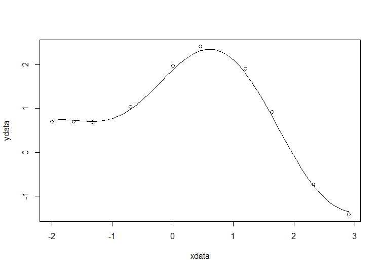
The R code used for this example comes from Barry Rowlingson, so huge thanks to him.
A question I get asked a lot is ‘How can I do nonlinear least squares curve fitting in X?’ where X might be MATLAB, Mathematica or a whole host of alternatives. Since this is such a common query, I thought I’d write up how to do it for a very simple problem in several systems that I’m interested in
This is the R version. For other versions,see the list below
- Simple nonlinear least squares curve fitting in Julia
- Simple nonlinear least squares curve fitting in Maple
- Simple nonlinear least squares curve fitting in Mathematica
- Simple nonlinear least squares curve fitting in MATLAB
- Simple nonlinear least squares curve fitting in Python
The problem
xdata = -2,-1.64,-1.33,-0.7,0,0.45,1.2,1.64,2.32,2.9
ydata = 0.699369,0.700462,0.695354,1.03905,1.97389,2.41143,1.91091,0.919576,-0.730975,-1.42001
and you’d like to fit the function

using nonlinear least squares. You’re starting guesses for the parameters are p1=1 and P2=0.2
For now, we are primarily interested in the following results:
- The fit parameters
- Sum of squared residuals
- Parameter confidence intervals
Future updates of these posts will show how to get other results. Let me know what you are most interested in.
Solution in R
# construct the data vectors using c()
xdata = c(-2,-1.64,-1.33,-0.7,0,0.45,1.2,1.64,2.32,2.9)
ydata = c(0.699369,0.700462,0.695354,1.03905,1.97389,2.41143,1.91091,0.919576,-0.730975,-1.42001)

# look at it
plot(xdata,ydata)

# some starting values
p1 = 1
p2 = 0.2

# do the fit
fit = nls(ydata ~ p1*cos(p2*xdata) + p2*sin(p1*xdata), start=list(p1=p1,p2=p2))

# summarise
summary(fit)
This gives
Formula: ydata ~ p1 * cos(p2 * xdata) + p2 * sin(p1 * xdata)

Parameters:
   Estimate Std. Error t value Pr(>|t|)
p1 1.881851   0.027430   68.61 2.27e-12 ***
p2 0.700230   0.009153   76.51 9.50e-13 ***
---
Signif. codes:  0 ‘***’ 0.001 ‘**’ 0.01 ‘*’ 0.05 ‘.’ 0.1 ‘ ’ 1

Residual standard error: 0.08202 on 8 degrees of freedom

Number of iterations to convergence: 7
Achieved convergence tolerance: 2.189e-06
Draw the fit on the plot by getting the prediction from the fit at 200 x-coordinates across the range of xdata
new = data.frame(xdata = seq(min(xdata),max(xdata),len=200))
lines(new$xdata,predict(fit,newdata=new))
Getting the sum of squared residuals is easy enough:
sum(resid(fit)^2)
Which gives
[1] 0.0538127
Finally, lets get the parameter confidence intervals.
confint(fit)
Which gives
Waiting for profiling to be done...
        2.5%     97.5%
p1 1.8206081 1.9442365
p2 0.6794193 0.7209843
A question I get asked a lot is ‘How can I do nonlinear least squares curve fitting in X?’ where X might be MATLAB, Mathematica or a whole host of alternatives. Since this is such a common query, I thought I’d write up how to do it for a very simple problem in several systems that I’m interested in
This is the MATLAB version. For other versions,see the list below
- Simple nonlinear least squares curve fitting in Julia
- Simple nonlinear least squares curve fitting in Maple
- Simple nonlinear least squares curve fitting in Mathematica
- Simple nonlinear least squares curve fitting in Python
- Simple nonlinear least squares curve fitting in R
The problem
xdata = -2,-1.64,-1.33,-0.7,0,0.45,1.2,1.64,2.32,2.9
ydata = 0.699369,0.700462,0.695354,1.03905,1.97389,2.41143,1.91091,0.919576,-0.730975,-1.42001
and you’d like to fit the function
using nonlinear least squares. You’re starting guesses for the parameters are p1=1 and P2=0.2
For now, we are primarily interested in the following results:
- The fit parameters
- Sum of squared residuals
Future updates of these posts will show how to get other results such as confidence intervals. Let me know what you are most interested in.
How you proceed depends on which toolboxes you have. Contrary to popular belief, you don’t need the Curve Fitting toolbox to do curve fitting…particularly when the fit in question is as basic as this. Out of the 90+ toolboxes sold by The Mathworks, I’ve only been able to look through the subset I have access to so I may have missed some alternative solutions.
Pure MATLAB solution (No toolboxes)
In order to perform nonlinear least squares curve fitting, you need to minimise the squares of the residuals. This means you need a minimisation routine. Basic MATLAB comes with the fminsearch function which is based on the Nelder-Mead simplex method. For this particular problem, it works OK but will not be suitable for more complex fitting problems. Here’s the code
format compact
format long
xdata = [-2,-1.64,-1.33,-0.7,0,0.45,1.2,1.64,2.32,2.9];
ydata = [0.699369,0.700462,0.695354,1.03905,1.97389,2.41143,1.91091,0.919576,-0.730975,-1.42001];

%Function to calculate the sum of residuals for a given p1 and p2
fun = @(p) sum((ydata - (p(1)*cos(p(2)*xdata)+p(2)*sin(p(1)*xdata))).^2);

%starting guess
pguess = [1,0.2];

%optimise
[p,fminres] = fminsearch(fun,pguess)
This gives the following results
p =
1.881831115804464 0.700242006994123
fminres =
0.053812720914713
All we get here are the parameters and the sum of squares of the residuals. If you want more information such as 95% confidence intervals, you’ll have a lot more hand-coding to do. Although fminsearch works fine in this instance, it soon runs out of steam for more complex problems.
MATLAB with optimisation toolbox
With respect to this problem, the optimisation toolbox gives you two main advantages over pure MATLAB. The first is that better optimisation routines are available so more complex problems (such as those with constraints) can be solved and in less time. The second is the provision of the lsqcurvefit function which is specifically designed to solve curve fitting problems. Here’s the code
format long
format compact
xdata = [-2,-1.64,-1.33,-0.7,0,0.45,1.2,1.64,2.32,2.9];
ydata = [0.699369,0.700462,0.695354,1.03905,1.97389,2.41143,1.91091,0.919576,-0.730975,-1.42001];

%Note that we don't have to explicitly calculate residuals
fun = @(p,xdata) p(1)*cos(p(2)*xdata)+p(2)*sin(p(1)*xdata);

%starting guess
pguess = [1,0.2];

[p,fminres] = lsqcurvefit(fun,pguess,xdata,ydata)
This gives the results
p =
   1.881848414551983   0.700229137656802
fminres =
   0.053812696487326
MATLAB with statistics toolbox
There are two interfaces I know of in the stats toolbox and both of them give a lot of information about the fit. The problem set up is the same in both cases
%set up for both fit commands in the stats toolbox
xdata = [-2,-1.64,-1.33,-0.7,0,0.45,1.2,1.64,2.32,2.9];
ydata = [0.699369,0.700462,0.695354,1.03905,1.97389,2.41143,1.91091,0.919576,-0.730975,-1.42001];

fun = @(p,xdata) p(1)*cos(p(2)*xdata)+p(2)*sin(p(1)*xdata);

pguess = [1,0.2];
Method 1 makes use of NonLinearModel.fit
mdl = NonLinearModel.fit(xdata,ydata,fun,pguess)
The returned object is a NonLinearModel object
class(mdl)
ans =
NonLinearModel
which contains all sorts of useful stuff
mdl =
Nonlinear regression model:
    y ~ p1*cos(p2*xdata) + p2*sin(p1*xdata)

Estimated Coefficients:
          Estimate             SE
    p1      1.8818508110535      0.027430139389359
    p2    0.700229815076442    0.00915260662357553

          tStat               pValue
    p1    68.6052223191956    2.26832562501304e-12
    p2    76.5060538352836    9.49546284187105e-13

Number of observations: 10, Error degrees of freedom: 8
Root Mean Squared Error: 0.082
R-Squared: 0.996,  Adjusted R-Squared 0.995
F-statistic vs. zero model: 1.43e+03, p-value = 6.04e-11
If you don’t need such heavyweight infrastructure, you can make use of the statistic toolbox’s nlinfit function
[p,R,J,CovB,MSE,ErrorModelInfo] = nlinfit(xdata,ydata,fun,pguess);
Along with our parameters (p) this also provides the residuals (R), Jacobian (J), Estimated variance-covariance matrix (CovB), Mean Squared Error (MSE) and a structure containing information about the error model fit (ErrorModelInfo).
Both nlinfit and NonLinearModel.fit use the same minimisation algorithm which is based on Levenberg-Marquardt
MATLAB with Symbolic Toolbox
MATLAB’s symbolic toolbox provides a completely separate computer algebra system called Mupad which can handle nonlinear least squares fitting via its stats::reg function. Here’s how to solve our problem in this environment.
First, you need to start up the mupad application. You can do this by entering
mupad
into MATLAB. Once you are in mupad, the code looks like this
xdata := [-2,-1.64,-1.33,-0.7,0,0.45,1.2,1.64,2.32,2.9]:
ydata := [0.699369,0.700462,0.695354,1.03905,1.97389,2.41143,1.91091,0.919576,-0.730975,-1.42001]:
stats::reg(xdata,ydata,p1*cos(p2*x)+p2*sin(p1*x),[x],[p1,p2],StartingValues=[1,0.2])
The result returned is
[[1.88185085, 0.7002298172], 0.05381269642]
These are our fitted parameters,p1 and p2, along with the sum of squared residuals. The documentation tells us that the optimisation algorithm is Levenberg-Marquardt– this is rather better than the simplex algorithm used by basic MATLAB’s fminsearch.
MATLAB with the NAG Toolbox
The NAG Toolbox for MATLAB is a commercial product offered by the UK based Numerical Algorithms Group. Their main products are their C and Fortran libraries but they also have a comprehensive MATLAB toolbox that contains something like 1500+ functions. My University has a site license for pretty much everything they put out and we make great use of it all. One of the benefits of the NAG toolbox over those offered by The Mathworks is speed. NAG is often (but not always) faster since its based on highly optimized, compiled Fortran. One of the problems with the NAG toolbox is that it is difficult to use compared to Mathworks toolboxes.
In an earlier blog post, I showed how to create wrappers for the NAG toolbox to create an easy to use interface for basic nonlinear curve fitting. Here’s how to solve our problem using those wrappers.
format long
format compact
xdata = [-2,-1.64,-1.33,-0.7,0,0.45,1.2,1.64,2.32,2.9];
ydata = [0.699369,0.700462,0.695354,1.03905,1.97389,2.41143,1.91091,0.919576,-0.730975,-1.42001];

%Note that we don't have to explicitly calculate residuals
fun = @(p,xdata) p(1)*cos(p(2)*xdata)+p(2)*sin(p(1)*xdata);
start = [1,0.2];
[p,fminres]=nag_lsqcurvefit(fun,start,xdata,ydata)
which gives
Warning: nag_opt_lsq_uncon_mod_func_easy (e04fy) returned a warning indicator (5)
p =
   1.881850904268710   0.700229557886739
fminres =
   0.053812696425390
For convenience, here’s the two files you’ll need to run the above (you’ll also need the NAG Toolbox for MATLAB of course)
MATLAB with curve fitting toolbox
One would expect the curve fitting toolbox to be able to fit such a simple curve and one would be right :)
xdata = [-2,-1.64,-1.33,-0.7,0,0.45,1.2,1.64,2.32,2.9];
ydata = [0.699369,0.700462,0.695354,1.03905,1.97389,2.41143,1.91091,0.919576,-0.730975,-1.42001];

opt = fitoptions('Method','NonlinearLeastSquares',...
               'Startpoint',[1,0.2]);
f = fittype('p1*cos(p2*x)+p2*sin(p1*x)','options',opt);

fitobject = fit(xdata',ydata',f)
Note that, unlike every other Mathworks method shown here, xdata and ydata have to be column vectors. The result looks like this
fitobject =

     General model:
     fitobject(x) = p1*cos(p2*x)+p2*sin(p1*x)
     Coefficients (with 95% confidence bounds):
       p1 =       1.882  (1.819, 1.945)
       p2 =      0.7002  (0.6791, 0.7213)
fitobject is of type cfit:
 class(fitobject)

ans =
cfit
In this case it contains two fields, p1 and p2, which are the parameters we are looking for
>> fieldnames(fitobject)
ans =
    'p1'
    'p2'
>> fitobject.p1
ans =
   1.881848414551983
>> fitobject.p2
ans =
    0.700229137656802
For maximum information, call the fit command like this:
[fitobject,gof,output] = fit(xdata',ydata',f)

fitobject =

     General model:
     fitobject(x) = p1*cos(p2*x)+p2*sin(p1*x)
     Coefficients (with 95% confidence bounds):
       p1 =       1.882  (1.819, 1.945)
       p2 =      0.7002  (0.6791, 0.7213)

gof =

           sse: 0.053812696487326
       rsquare: 0.995722238905101
           dfe: 8
    adjrsquare: 0.995187518768239
          rmse: 0.082015773244637

output =

           numobs: 10
         numparam: 2
        residuals: [10x1 double]
         Jacobian: [10x2 double]
         exitflag: 3
    firstorderopt: 3.582047395989108e-05
       iterations: 6
        funcCount: 21
     cgiterations: 0
        algorithm: 'trust-region-reflective'
          message: [1x86 char]
A question I get asked a lot is ‘How can I do nonlinear least squares curve fitting in X?’ where X might be MATLAB, Mathematica or a whole host of alternatives. Since this is such a common query, I thought I’d write up how to do it for a very simple problem in several systems that I’m interested in
This is the Maple version. For other versions,see the list below
- Simple nonlinear least squares curve fitting in Julia
- Simple nonlinear least squares curve fitting in Mathematica
- Simple nonlinear least squares curve fitting in MATLAB
- Simple nonlinear least squares curve fitting in Python
- Simple nonlinear least squares curve fitting in R
The problem
xdata = -2,-1.64,-1.33,-0.7,0,0.45,1.2,1.64,2.32,2.9
ydata = 0.699369,0.700462,0.695354,1.03905,1.97389,2.41143,1.91091,0.919576,-0.730975,-1.42001
and you’d like to fit the function
using nonlinear least squares. You’re starting guesses for the parameters are p1=1 and P2=0.2
For now, we are primarily interested in the following results:
- The fit parameters
- Sum of squared residuals
Future updates of these posts will show how to get other results such as confidence intervals. Let me know what you are most interested in.
Solution in Maple
Maple’s user interface is quite user friendly and it uses non-linear optimization routines from The Numerical Algorithms Group under the hood. Here’s the code to get the parameter values and sum of squares of residuals
with(Statistics):

xdata := Vector([-2, -1.64, -1.33, -.7, 0, .45, 1.2, 1.64, 2.32, 2.9], datatype = float):
ydata := Vector([.699369, .700462, .695354, 1.03905, 1.97389, 2.41143, 1.91091, .919576,
  -.730975, -1.42001], datatype = float):
NonlinearFit(p1*cos(p2*x)+p2*sin(p1*x), xdata, ydata, x, initialvalues = [p1 = 1, p2 = .2],
   output = [parametervalues, residualsumofsquares])
which gives the result
[[p1 = 1.88185090465902, p2 = 0.700229557992540], 0.05381269642]
Various other outputs can be specified in the output vector such as:
- solutionmodule
- degreesoffreedom
- leastsquaresfunction
- parametervalues
- parametervector
- residuals
- residualmeansquare
- residualstandarddeviation
- residualsumofsquares.
The meanings of the above are mostly obvious. In those cases where they aren’t, you can look them up in the documentation link below.
Further documentation
The full documentation for Maple’s NonlinearFit command is at http://www.maplesoft.com/support/help/Maple/view.aspx?path=Statistics%2fNonlinearFit
Notes
I used Maple 17.02 on 64bit Windows to run the code in this post.
A question I get asked a lot is ‘How can I do nonlinear least squares curve fitting in X?’ where X might be MATLAB, Mathematica or a whole host of alternatives. Since this is such a common query, I thought I’d write up how to do it for a very simple problem in several systems that I’m interested in
This is the Python version. For other versions,see the list below
- Simple nonlinear least squares curve fitting in Julia
- Simple nonlinear least squares curve fitting in Maple
- Simple nonlinear least squares curve fitting in Mathematica
- Simple nonlinear least squares curve fitting in MATLAB
- Simple nonlinear least squares curve fitting in R
The problem
xdata = -2,-1.64,-1.33,-0.7,0,0.45,1.2,1.64,2.32,2.9
ydata = 0.699369,0.700462,0.695354,1.03905,1.97389,2.41143,1.91091,0.919576,-0.730975,-1.42001
and you’d like to fit the function
using nonlinear least squares. You’re starting guesses for the parameters are p1=1 and P2=0.2
For now, we are primarily interested in the following results:
- The fit parameters
- Sum of squared residuals
Future updates of these posts will show how to get other results such as confidence intervals. Let me know what you are most interested in.
Python solution using scipy
Here, I use the curve_fit function from scipy
import numpy as np
from scipy.optimize import curve_fit

xdata = np.array([-2,-1.64,-1.33,-0.7,0,0.45,1.2,1.64,2.32,2.9])
ydata = np.array([0.699369,0.700462,0.695354,1.03905,1.97389,2.41143,1.91091,0.919576,-0.730975,-1.42001])

def func(x, p1,p2):
  return p1*np.cos(p2*x) + p2*np.sin(p1*x)

popt, pcov = curve_fit(func, xdata, ydata,p0=(1.0,0.2))
The variable popt contains the fit parameters
array([ 1.88184732, 0.70022901])
We need to do a little more work to get the sum of squared residuals
p1 = popt[0]
p2 = popt[1]
residuals = ydata - func(xdata,p1,p2)
fres = sum(residuals**2)
which gives
0.053812696547933969
- I’ve put this in an Ipython notebook which can be downloaded here. There is also a pdf version of the notebook.
A question I get asked a lot is ‘How can I do nonlinear least squares curve fitting in X?’ where X might be MATLAB, Mathematica or a whole host of alternatives. Since this is such a common query, I thought I’d write up how to do it for a very simple problem in several systems that I’m interested in
This is the Mathematica version. For other versions,see the list below
- Simple nonlinear least squares curve fitting in Maple
- Simple nonlinear least squares curve fitting in Julia
- Simple nonlinear least squares curve fitting in MATLAB
- Simple nonlinear least squares curve fitting in Python
- Simple nonlinear least squares curve fitting in R
The problem
You have the following 10 data points
xdata = -2,-1.64,-1.33,-0.7,0,0.45,1.2,1.64,2.32,2.9
ydata = 0.699369,0.700462,0.695354,1.03905,1.97389,2.41143,1.91091,0.919576,-0.730975,-1.42001
and you’d like to fit the function
using nonlinear least squares. You’re starting guesses for the parameters are p1=1 and P2=0.2
For now, we are primarily interested in the following results:
- The fit parameters
- Sum of squared residuals
Future updates of these posts will show how to get other results such as confidence intervals. Let me know what you are most interested in.
Mathematica Solution using FindFit
FindFit is the basic nonlinear curve fitting routine in Mathematica
xdata={-2,-1.64,-1.33,-0.7,0,0.45,1.2,1.64,2.32,2.9};
ydata={0.699369,0.700462,0.695354,1.03905,1.97389,2.41143,1.91091,0.919576,-0.730975,-1.42001};

(*Mathematica likes to have the data in the form {{x1,y1},{x2,y2},..}*)
data = Partition[Riffle[xdata, ydata], 2];

FindFit[data, p1*Cos[p2 x] + p2*Sin[p1 x], {{p1, 1}, {p2, 0.2}}, x]

Out[4]:={p1->1.88185,p2->0.70023}
Mathematica Solution using NonlinearModelFit
You can get a lot more information about the fit using the NonLinearModelFit function
(*Set up data as before*)
xdata={-2,-1.64,-1.33,-0.7,0,0.45,1.2,1.64,2.32,2.9};
ydata={0.699369,0.700462,0.695354,1.03905,1.97389,2.41143,1.91091,0.919576,-0.730975,-1.42001};
data = Partition[Riffle[xdata, ydata], 2];

(*Create the NonLinearModel object*)
nlm = NonlinearModelFit[data, p1*Cos[p2 x] + p2*Sin[p1 x], {{p1, 1}, {p2, 0.2}}, x];
The NonLinearModel object contains many properties that may be useful to us. Here’s how to list them all
nlm["Properties"]

Out[10]= {"AdjustedRSquared", "AIC", "AICc", "ANOVATable", \
"ANOVATableDegreesOfFreedom", "ANOVATableEntries", "ANOVATableMeanSquares", \
"ANOVATableSumsOfSquares", "BestFit", "BestFitParameters", "BIC", \
"CorrelationMatrix", "CovarianceMatrix", "CurvatureConfidenceRegion", "Data", \
"EstimatedVariance", "FitCurvatureTable", "FitCurvatureTableEntries", \
"FitResiduals", "Function", "HatDiagonal", "MaxIntrinsicCurvature", \
"MaxParameterEffectsCurvature", "MeanPredictionBands", \
"MeanPredictionConfidenceIntervals", "MeanPredictionConfidenceIntervalTable", \
"MeanPredictionConfidenceIntervalTableEntries", "MeanPredictionErrors", \
"ParameterBias", "ParameterConfidenceIntervals", \
"ParameterConfidenceIntervalTable", \
"ParameterConfidenceIntervalTableEntries", "ParameterConfidenceRegion", \
"ParameterErrors", "ParameterPValues", "ParameterTable", \
"ParameterTableEntries", "ParameterTStatistics", "PredictedResponse", \
"Properties", "Response", "RSquared", "SingleDeletionVariances", \
"SinglePredictionBands", "SinglePredictionConfidenceIntervals", \
"SinglePredictionConfidenceIntervalTable", \
"SinglePredictionConfidenceIntervalTableEntries", "SinglePredictionErrors", \
"StandardizedResiduals", "StudentizedResiduals"}
Let’s extract the fit parameters, 95% confidence levels and residuals
{params, confidenceInt, res} =
 nlm[{"BestFitParameters", "ParameterConfidenceIntervals", "FitResiduals"}]

Out[22]= {{p1 -> 1.88185,
  p2 -> 0.70023}, {{1.8186, 1.9451}, {0.679124,
   0.721336}}, {-0.0276906, -0.0322944, -0.0102488, 0.0566244,
  0.0920392, 0.0976307, 0.114035, 0.109334, 0.0287154, -0.0700442}}
The parameters are given as replacement rules. Here, we convert them to pure numbers
{p1, p2} = {p1, p2} /. params

Out[38]= {1.88185,0.70023}
Although only a few decimal places are shown, p1 and p2 are stored in full double precision. You can see this by converting to InputForm
InputForm[{p1, p2}]

Out[43]//InputForm=
{1.8818508498053645, 0.7002298171759191}
Similarly, let’s look at the 95% confidence interval, extracted earlier, in full precision
confidenceInt // InputForm

Out[44]//InputForm=
{{1.8185969887307214, 1.9451047108800077},
 {0.6791239458086734, 0.7213356885431649}}
Calculate the sum of squared residuals
resnorm = Total[res^2]

Out[45]= 0.0538127
Notes
I used Mathematica 9 on Windows 7 64bit to perform these calculations
As soon as I heard the news that Mathematica was being made available completely free on the Raspberry Pi, I just had to get myself a Pi and have a play. So, I bought the Raspberry Pi Advanced Kit from my local Maplin Electronics store, plugged it to the kitchen telly and booted it up. The exercise made me miss my father because the last time I plugged a computer into the kitchen telly was when I was 8 years old; it was Christmas morning and dad and I took our first steps into a new world with my Sinclair Spectrum 48K.
How to install Mathematica on the Raspberry Pi
Future raspberry pis wll have Mathematica installed by default but mine wasn’t new enough so I just typed the following at the command line
sudo apt-get update && sudo apt-get install wolfram-engine
On my machine, I was told
The following extra packages will be installed:
  oracle-java7-jdk
The following NEW packages will be installed:
  oracle-java7-jdk wolfram-engine
0 upgraded, 2 newly installed, 0 to remove and 1 not upgraded.
Need to get 278 MB of archives.
After this operation, 588 MB of additional disk space will be used.
So, it seems that Mathematica needs Oracle’s Java and that’s being installed for me as well. The combination of the two is going to use up 588MB of disk space which makes me glad that I have an 8Gb SD card in my pi.
Mathematica version 10!
On starting Mathematica on the pi, my first big surprise was the version number. I am the administrator of an unlimited academic site license for Mathematica at The University of Manchester and the latest version we can get for our PCs at the time of writing is 9.0.1. My free pi version is at version 10! The first clue is the installation directory:
/opt/Wolfram/WolframEngine/10.0
and the next clue is given by evaluating $Version in Mathematica itself
In[2]:= $Version

Out[2]= "10.0 for Linux ARM (32-bit) (November 19, 2013)"
To get an idea of what’s new in 10, I evaluated the following command on Mathematica on the Pi
Export["PiFuncs.dat",Names["System`*"]]
This creates a PiFuncs.dat file which tells me the list of functions in the System context on the version of Mathematica on the pi. Transfer this over to my Windows PC and import into Mathematica 9.0.1 with
pifuncs = Flatten[Import["PiFuncs.dat"]];
Get the list of functions from version 9.0.1 on Windows:
winVer9funcs = Names["System`*"];
Finally, find out what’s in pifuncs but not winVer9funcs
In[16]:= Complement[pifuncs, winVer9funcs]
Out[16]= {"Activate", "AffineStateSpaceModel", "AllowIncomplete", \
"AlternatingFactorial", "AntihermitianMatrixQ", \
"AntisymmetricMatrixQ", "APIFunction", "ArcCurvature", "ARCHProcess", \
"ArcLength", "Association", "AsymptoticOutputTracker", \
"AutocorrelationTest", "BarcodeImage", "BarcodeRecognize", \
"BoxObject", "CalendarConvert", "CanonicalName", "CantorStaircase", \
"ChromaticityPlot", "ClassifierFunction", "Classify", \
"ClipPlanesStyle", "CloudConnect", "CloudDeploy", "CloudDisconnect", \
"CloudEvaluate", "CloudFunction", "CloudGet", "CloudObject", \
"CloudPut", "CloudSave", "ColorCoverage", "ColorDistance", "Combine", \
"CommonName", "CompositeQ", "Computed", "ConformImages", "ConformsQ", \
"ConicHullRegion", "ConicHullRegion3DBox", "ConicHullRegionBox", \
"ConstantImage", "CountBy", "CountedBy", "CreateUUID", \
"CurrencyConvert", "DataAssembly", "DatedUnit", "DateFormat", \
"DateObject", "DateObjectQ", "DefaultParameterType", \
"DefaultReturnType", "DefaultView", "DeviceClose", "DeviceConfigure", \
"DeviceDriverRepository", "DeviceExecute", "DeviceInformation", \
"DeviceInputStream", "DeviceObject", "DeviceOpen", "DeviceOpenQ", \
"DeviceOutputStream", "DeviceRead", "DeviceReadAsynchronous", \
"DeviceReadBuffer", "DeviceReadBufferAsynchronous", \
"DeviceReadTimeSeries", "Devices", "DeviceWrite", \
"DeviceWriteAsynchronous", "DeviceWriteBuffer", \
"DeviceWriteBufferAsynchronous", "DiagonalizableMatrixQ", \
"DirichletBeta", "DirichletEta", "DirichletLambda", "DSolveValue", \
"Entity", "EntityProperties", "EntityProperty", "EntityValue", \
"Enum", "EvaluationBox", "EventSeries", "ExcludedPhysicalQuantities", \
"ExportForm", "FareySequence", "FeedbackLinearize", "Fibonorial", \
"FileTemplate", "FileTemplateApply", "FindAllPaths", "FindDevices", \
"FindEdgeIndependentPaths", "FindFundamentalCycles", \
"FindHiddenMarkovStates", "FindSpanningTree", \
"FindVertexIndependentPaths", "Flattened", "ForeignKey", \
"FormatName", "FormFunction", "FormulaData", "FormulaLookup", \
"FractionalGaussianNoiseProcess", "FrenetSerretSystem", "FresnelF", \
"FresnelG", "FullInformationOutputRegulator", "FunctionDomain", \
"FunctionRange", "GARCHProcess", "GeoArrow", "GeoBackground", \
"GeoBoundaryBox", "GeoCircle", "GeodesicArrow", "GeodesicLine", \
"GeoDisk", "GeoElevationData", "GeoGraphics", "GeoGridLines", \
"GeoGridLinesStyle", "GeoLine", "GeoMarker", "GeoPoint", \
"GeoPolygon", "GeoProjection", "GeoRange", "GeoRangePadding", \
"GeoRectangle", "GeoRhumbLine", "GeoStyle", "Graph3D", "GroupBy", \
"GroupedBy", "GrowCutBinarize", "HalfLine", "HalfPlane", \
"HiddenMarkovProcess", "ï¯", "ï ", "ï ", "ï ", "ï ", "ï ", \
"ï
", "ï ", "ï ", "ï ", "ï ", "ï ", "ï ", "ï ", "ï ", "ï ", \
"ï ", "ï ", "ï ", "ï ", "ï ", "ï ", "ï ", "ï ", "ï ", "ï ", \
"ï ", "ï ", "ï ", "ï ", "ï ", "ï ", "ï ", "ï ", "ï ¦", "ï ª", \
"ï ¯", "ï \.b2", "ï \.b3", "IgnoringInactive", "ImageApplyIndexed", \
"ImageCollage", "ImageSaliencyFilter", "Inactivate", "Inactive", \
"IncludeAlphaChannel", "IncludeWindowTimes", "IndefiniteMatrixQ", \
"IndexedBy", "IndexType", "InduceType", "InferType", "InfiniteLine", \
"InfinitePlane", "InflationAdjust", "InflationMethod", \
"IntervalSlider", "ï ¨", "ï ¢", "ï ©", "ï ¤", "ï \[Degree]", "ï ", \
"ï ¡", "ï «", "ï ®", "ï §", "ï £", "ï ¥", "ï \[PlusMinus]", \
"ï \[Not]", "JuliaSetIterationCount", "JuliaSetPlot", \
"JuliaSetPoints", "KEdgeConnectedGraphQ", "Key", "KeyDrop", \
"KeyExistsQ", "KeyIntersection", "Keys", "KeySelect", "KeySort", \
"KeySortBy", "KeyTake", "KeyUnion", "KillProcess", \
"KVertexConnectedGraphQ", "LABColor", "LinearGradientImage", \
"LinearizingTransformationData", "ListType", "LocalAdaptiveBinarize", \
"LocalizeDefinitions", "LogisticSigmoid", "Lookup", "LUVColor", \
"MandelbrotSetIterationCount", "MandelbrotSetMemberQ", \
"MandelbrotSetPlot", "MinColorDistance", "MinimumTimeIncrement", \
"MinIntervalSize", "MinkowskiQuestionMark", "MovingMap", \
"NegativeDefiniteMatrixQ", "NegativeSemidefiniteMatrixQ", \
"NonlinearStateSpaceModel", "Normalized", "NormalizeType", \
"NormalMatrixQ", "NotebookTemplate", "NumberLinePlot", "OperableQ", \
"OrthogonalMatrixQ", "OverwriteTarget", "PartSpecification", \
"PlotRangeClipPlanesStyle", "PositionIndex", \
"PositiveSemidefiniteMatrixQ", "Predict", "PredictorFunction", \
"PrimitiveRootList", "ProcessConnection", "ProcessInformation", \
"ProcessObject", "ProcessStatus", "Qualifiers", "QuantityVariable", \
"QuantityVariableCanonicalUnit", "QuantityVariableDimensions", \
"QuantityVariableIdentifier", "QuantityVariablePhysicalQuantity", \
"RadialGradientImage", "RandomColor", "RegularlySampledQ", \
"RemoveBackground", "RequiredPhysicalQuantities", "ResamplingMethod", \
"RiemannXi", "RSolveValue", "RunProcess", "SavitzkyGolayMatrix", \
"ScalarType", "ScorerGi", "ScorerGiPrime", "ScorerHi", \
"ScorerHiPrime", "ScriptForm", "Selected", "SendMessage", \
"ServiceConnect", "ServiceDisconnect", "ServiceExecute", \
"ServiceObject", "ShowWhitePoint", "SourceEntityType", \
"SquareMatrixQ", "Stacked", "StartDeviceHandler", "StartProcess", \
"StateTransformationLinearize", "StringTemplate", "StructType", \
"SystemGet", "SystemsModelMerge", "SystemsModelVectorRelativeOrder", \
"TemplateApply", "TemplateBlock", "TemplateExpression", "TemplateIf", \
"TemplateObject", "TemplateSequence", "TemplateSlot", "TemplateWith", \
"TemporalRegularity", "ThermodynamicData", "ThreadDepth", \
"TimeObject", "TimeSeries", "TimeSeriesAggregate", \
"TimeSeriesInsert", "TimeSeriesMap", "TimeSeriesMapThread", \
"TimeSeriesModel", "TimeSeriesModelFit", "TimeSeriesResample", \
"TimeSeriesRescale", "TimeSeriesShift", "TimeSeriesThread", \
"TimeSeriesWindow", "TimeZoneConvert", "TouchPosition", \
"TransformedProcess", "TrapSelection", "TupleType", "TypeChecksQ", \
"TypeName", "TypeQ", "UnitaryMatrixQ", "URLBuild", "URLDecode", \
"URLEncode", "URLExistsQ", "URLExpand", "URLParse", "URLQueryDecode", \
"URLQueryEncode", "URLShorten", "ValidTypeQ", "ValueDimensions", \
"Values", "WhiteNoiseProcess", "XMLTemplate", "XYZColor", \
"ZoomLevel", "$CloudBase", "$CloudConnected", "$CloudDirectory", \
"$CloudEvaluation", "$CloudRootDirectory", "$EvaluationEnvironment", \
"$GeoLocationCity", "$GeoLocationCountry", "$GeoLocationPrecision", \
"$GeoLocationSource", "$RegisteredDeviceClasses", \
"$RequesterAddress", "$RequesterWolframID", "$RequesterWolframUUID", \
"$UserAgentLanguages", "$UserAgentMachine", "$UserAgentName", \
"$UserAgentOperatingSystem", "$UserAgentString", "$UserAgentVersion", \
"$WolframID", "$WolframUUID"}
There we have it, a preview of the list of functions that might be coming in desktop version 10 of Mathematica courtesy of the free Pi version.
No local documentation
On a desktop version of Mathematica, all of the Mathematica documentation is available on your local machine by clicking on Help->Documentation Center in the Mathematica notebook interface. On the pi version, it seems that there is no local documentation, presumably to keep the installation size down. You get to the documentation via the notebook interface by clicking on Help->OnlineDocumentation which takes you to http://reference.wolfram.com/language/?src=raspi
Speed vs my laptop
I am used to running Mathematica on high specification machines and so naturally the pi version felt very sluggish–particularly when using the notebook interface. With that said, however, I found it very usable for general playing around. I was very curious, however, about the speed of the pi version compared to the version on my home laptop and so created a small benchmark notebook that did three things:
- Calculate pi to 1,000,000 decimal places.
- Multiply two 1000 x 1000 random matrices together
- Integrate sin(x)^2*tan(x) with respect to x
The comparison is going to be against my Windows 7 laptop which has a quad-core Intel Core i7-2630QM. The procedure I followed was:
- Start a fresh version of the Mathematica notebook and open pi_bench.nb
- Click on Evaluation->Evaluate Notebook and record the times
- Click on Evaluation->Evaluate Notebook again and record the new times.
Note that I use the AbsoluteTiming function instead of Timing (detailed reason given here) and I clear the system cache (detailed resason given here). You can download the notebook I used here. Alternatively, copy and paste the code below
(*Clear Cache*)
ClearSystemCache[]

(*Calculate pi to 1 million decimal places and store the result*)
AbsoluteTiming[pi = N[Pi, 1000000];]

(*Multiply two random 1000x1000 matrices together and store the \
result*)
a = RandomReal[1, {1000, 1000}];
b = RandomReal[1, {1000, 1000}];

AbsoluteTiming[prod = Dot[a, b];]

(*calculate an integral and store the result*)
AbsoluteTiming[res = Integrate[Sin[x]^2*Tan[x], x];]
Here are the results. All timings in seconds.
| Test | Laptop Run 1 | Laptop Run 2 | RaspPi Run 1 | RaspPi Run 2 | Best Pi/Best Laptop |
| Million digits of Pi | 0.994057 | 1.007058 | 14.101360 | 13.860549 | 13.9434 |
| Matrix product | 0.108006 | 0.074004 | 85.076986 | 85.526180 | 1149.63 |
| Symbolic integral | 0.035002 | 0.008000 | 0.980086 | 0.448804 | 56.1 |
From these tests, we see that Mathematica on the pi is around 14 to 1149 times slower on the pi than my laptop. The huge difference between the pi and laptop for the matrix product stems from the fact that ,on the laptop, Mathematica is using Intels Math Kernel Library (MKL). The MKL is extremely well optimised for Intel processors and will be using all 4 of the laptop’s CPU cores along with extra tricks such as AVX operations etc. I am not sure what is being used on the pi for this operation.
I also ran the standard BenchMarkReport[] on the Raspberry Pi. The results are available here.
Speed vs Python
Comparing Mathematica on the pi to Mathematica on my laptop might have been a fun exercise for me but it’s not really fair on the pi which wasn’t designed to perform against expensive laptops. So, let’s move on to a more meaningful speed comparison: Mathematica on pi versus Python on pi.
When it comes to benchmarking on Python, I usually turn to the timeit module. This time, however, I’m not going to use it and that’s because of something odd that’s happening with sympy and caching. I’m using sympy to calculate pi to 1 million places and for the symbolic calculus. Check out this ipython session on the pi
pi@raspberrypi ~ $ SYMPY_USE_CACHE=no
pi@raspberrypi ~ $ ipython
Python 2.7.3 (default, Jan 13 2013, 11:20:46)
Type "copyright", "credits" or "license" for more information.

IPython 0.13.1 -- An enhanced Interactive Python.
?         -> Introduction and overview of IPython's features.
%quickref -> Quick reference.
help      -> Python's own help system.
object?   -> Details about 'object', use 'object??' for extra details.

In [1]: import sympy
In [2]: pi=sympy.pi.evalf(100000) #Takes a few seconds
In [3]: %timeit pi=sympy.pi.evalf(100000)
100 loops, best of 3: 2.35 ms per loop
In short, I have asked sympy not to use caching (I think!) and yet it is caching the result. I don’t want to time how quickly sympy can get a result from the cache so I can’t use timeit until I figure out what’s going on here. Since I wanted to publish this post sooner rather than later I just did this:
import sympy
import time
import numpy

start = time.time()
pi=sympy.pi.evalf(1000000)
elapsed = (time.time() - start)
print('1 million pi digits: %f seconds' % elapsed)

a = numpy.random.uniform(0,1,(1000,1000))
b = numpy.random.uniform(0,1,(1000,1000))
start = time.time()
c=numpy.dot(a,b)
elapsed = (time.time() - start)
print('Matrix Multiply: %f seconds' % elapsed)

x=sympy.Symbol('x')
start = time.time()
res=sympy.integrate(sympy.sin(x)**2*sympy.tan(x),x)
elapsed = (time.time() - start)
print('Symbolic Integration: %f seconds' % elapsed)
Usually, I’d use time.clock() to measure things like this but something *very* strange is happening with time.clock() on my pi–something I’ll write up later. In short, it didn’t work properly and so I had to resort to time.time().
Here are the results:
1 million pi digits: 5535.621769 seconds
Matrix Multiply: 77.938481 seconds
Symbolic Integration: 1654.666123 seconds
The result that really surprised me here was the symbolic integration since the problem I posed didn’t look very difficult. Sympy on pi was thousands of times slower than Mathematica on pi for this calculation! On my laptop, the calculation times between Mathematica and sympy were about the same for this operation.
That Mathematica beats sympy for 1 million digits of pi doesn’t surprise me too much since I recall attending a seminar a few years ago where Wolfram Research described how they had optimized the living daylights out of that particular operation. Nice to see Python beating Mathematica by a little bit in the linear algebra though.
Last week I gave a live demo of the IPython notebook to a group of numerical analysts and one of the computations we attempted to do was to solve the following linear system using Numpy’s solve command.

Now, the matrix shown above is singular and so we expect that we might have problems. Before looking at how Numpy deals with this computation, lets take a look at what happens if you ask MATLAB to do it
>> A=[1 2 3;4 5 6;7 8 9];
>> b=[15;15;15];
>> x=A\b
Warning: Matrix is close to singular
or badly scaled. Results may be
inaccurate. RCOND =  1.541976e-18.
x =
  -39.0000
   63.0000
  -24.0000
MATLAB gives us a warning that the input matrix is close to being singular (note that it didn’t actually recognize that it is singular) along with an estimate of the reciprocal of the condition number. It tells us that the results may be inaccurate and we’d do well to check. So, lets check:
>> A*x

ans =
   15.0000
   15.0000
   15.0000

>> norm(A*x-b)

ans =
2.8422e-14
We seem to have dodged the bullet since, despite the singular nature of our matrix, MATLAB has able to find a valid solution. MATLAB was right to have warned us though…in other cases we might not have been so lucky.
Let’s see how Numpy deals with this using the IPython notebook:
In [1]:
import numpy
from numpy import array
from numpy.linalg import solve
A=array([[1,2,3],[4,5,6],[7,8,9]])
b=array([15,15,15])
solve(A,b)

Out[1]:

array([-39.,  63., -24.])
It gave the same result as MATLAB [See note 1], presumably because it’s using the exact same LAPACK routine, but there was no warning of the singular nature of the matrix. During my demo, it was generally felt by everyone in the room that a warning should have been given, particularly when working in an interactive setting.
If you look at the documentation for Numpy’s solve command you’ll see that it is supposed to throw an exception when the matrix is singular but it clearly didn’t do so here. The exception is sometimes thrown though:
In [4]:

C=array([[1,1,1],[1,1,1],[1,1,1]])
x=solve(C,b)

---------------------------------------------------------------------------
LinAlgError                               Traceback (most recent call last)
 in ()
      1 C=array([[1,1,1],[1,1,1],[1,1,1]])
----> 2 x=solve(C,b)

C:\Python32\lib\site-packages\numpy\linalg\linalg.py in solve(a, b)
    326     results = lapack_routine(n_eq, n_rhs, a, n_eq, pivots, b, n_eq, 0)
    327     if results['info'] > 0:
--> 328         raise LinAlgError('Singular matrix')
    329     if one_eq:
    330         return wrap(b.ravel().astype(result_t))

LinAlgError: Singular matrix
It seems that Numpy is somehow checking for exact singularity but this will rarely be detected due to rounding errors. Those I’ve spoken to consider that MATLAB’s approach of estimating the condition number and warning when that is high would be better behavior since it alerts the user to the fact that the matrix is badly conditioned.
Thanks to Nick Higham and David Silvester for useful discussions regarding this post.
Notes
[1] – The results really are identical which you can see by rerunning the calculation after evaluating format long in MATLAB and numpy.set_printoptions(precision=15) in Python
Right now it’s packaging season (not the official term!) at my university–a time of year when IT staff have to battle with silent installers, SCCM, MSI creation and Adminstudio in order to create the student desktop image for the next academic year. Packaging season makes me grouchy, it makes me work late and it makes me massively over-react to every minor installation issue caused by software vendors. Right now, however, I am not grouchy because of packaging season..I am grouchy because of concurrent network licensing (or floating licensing if you are Wikipedia).
I like network licenses…they make many aspects of my job easier but they the way they are implemented by some software vendors causes them to be a pain. Over the years, I’ve bothered many a support-desk with my network license tails of woe and thought that I would collate them all together in one blog post.
The more of these things your software does, the more pain you cause me and my colleagues.
1. You don’t use standard FlexLM/FlexNet.
Like it or loathe it, FlexLM is used by the vast majority of software vendors out there. We run license servers that host dozens of FlexLM based applications and we have got the administration of these down to a fine art. In fact, we’ve replaced the vast majority of the process with a script. If an application uses FlexLM, system administration and license monitoring is bordering on the trivial for us now. The further you stray away from FlexLM, the more difficult our job becomes.
One thing guaranteed to ruin my day is a call from a vendor I’ve worked with for years who says ‘Great news Mike, we’re ditching FlexLM for our own, in house license system.’ Fabulous! Rather than use our lovely, generic, one-size fits all scripts, we are going to have to do a load of extra work and testing just for you. I look forward to all the new and interesting bugs your system will generate.
2. You don’t support redundant license servers.
The idea behind redundant license servers is this: Instead of your application relying on just one machine, it relies on three; only two of which have to be operational at any one time. This gives us resiliency and resiliency is a good thing when you are teaching a lab with 120 students in it.
I’ll keep this simple. If you don’t support redundant license servers, it means that you don’t believe that your software is important. It tells me that you are just playing at being a big, grown up piece of software but you don’t really think anyone will take you seriously.
3. You support redundant license servers but can’t select them via the installer.
At install time, there is no option to give three severs. The user can only give one. You then expect the user to copy a pre-prepared license file that has details of all three servers as a post-installation step.
What usually happens here is that users give the primary license server, find that the application will launch and stop reading the installation instructions. At some point in the future, we take down the primary license server for maintenance and the vast majority of self-serve installations break!
4. You use the LM_LICENSE_FILE environment variable
The problem is, so does everyone else. We end up with a situation where the LM_LICENSE_FILE variable is pointing at several license servers and some client applications really don’t like that. Be a good FlexLM citizen and use a vendor specific environment variable. For example, MATLAB uses MLM_LICENSE_FILE and I could give them a big hug just for that!
5. You ‘helpfully’ tell the user when the license is about to expire.
I’ve moaned about this before. 1000 users panicking and emailing the helpdesk…lovely! Bonus points are awarded if you don’t allow any supported way of switching these warnings off.
6. Your new license doesn’t support old clients.
This should speak for itself and happens more than I’d like. We can’t upgrade the entire estate instantaneously and even if we could, we probably wouldn’t want to. Some users, for one reason or another, cling to old versions of your software like grim death. They don’t care that there is a new shiny version available, all they know is that I broke their application and they hate me for it.
When we discover that old versions of your application will stop working, it also delays roll out of the new version since we have to do a lot of user-communications and ensure that nothing mission-critical will stop working. This makes power-users of your application hate me because they want the new shiny version.
7. You don’t have a silent installer.
Strictly speaking not a network license moan but closely related. We use network licensing because we deploy your software to lots of machines. When I say ‘lots’ I mean thousands. It turns out, however, that you don’t support scripted installation (sometimes called ‘silent installation’ or ‘unattended installation’). This means that your software is a lot more difficult to deploy than your competitor! I’m now a big fan of your competitor!
8. You have a silent installer but it’s a bad one.
If I install manually, via point and click, I can configure every aspect of your application. Your silent installer, on the other hand, is just a /S switch that does a default install…no configuration possible. Bonus points for ‘silent’ installers that include pop-up dialogue boxes that can’t be switched off.
While on the topic of silent installation, can I just ask that you directly support deployment by SCCM on Windows please? It will help with next year’s packaging season big time!
Cheers,
Mike
The first stable version of KryPy was released in late July. KryPy is “a Python module for Krylov subspace methods for the solution of linear algebraic systems. This includes enhanced versions of CG, MINRES and GMRES as well as methods for the efficient solution of sequences of linear systems.”
Here’s a toy example taken from KryPy’s website that shows how easy it is to use.
from numpy import ones
from scipy.sparse import spdiags
from krypy.linsys import gmres

N = 10
A = spdiags(range(1,N+1), [0], N, N)
b = ones((N,1))

sol = gmres(A, b)
print (sol['relresvec'])
Thanks to KryPy’s author, André Gaul, for the news.