Walking Randomly

The R code used for this example comes from Barry Rowlingson, so huge thanks to him.

A question I get asked a lot is ‘How can I do nonlinear least squares curve fitting in X?’ where X might be MATLAB, Mathematica or a whole host of alternatives.  Since this is such a common query, I thought I’d write up how to do it for a very simple problem in several systems that I’m interested in

This is the R version. For other versions,see the list below

• Simple nonlinear least squares curve fitting in Julia
• Simple nonlinear least squares curve fitting in Maple
• Simple nonlinear least squares curve fitting in Mathematica
• Simple nonlinear least squares curve fitting in MATLAB
• Simple nonlinear least squares curve fitting in Python

The problem

xdata = -2,-1.64,-1.33,-0.7,0,0.45,1.2,1.64,2.32,2.9
ydata = 0.699369,0.700462,0.695354,1.03905,1.97389,2.41143,1.91091,0.919576,-0.730975,-1.42001

and you’d like to fit the function

using nonlinear least squares.  You’re starting guesses for the parameters are p1=1 and P2=0.2

For now, we are primarily interested in the following results:

• The fit parameters
• Sum of squared residuals
• Parameter confidence intervals

Future updates of these posts will show how to get other results. Let me know what you are most interested in.

Solution in R

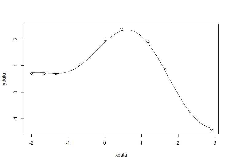
# construct the data vectors using c()
xdata = c(-2,-1.64,-1.33,-0.7,0,0.45,1.2,1.64,2.32,2.9)
ydata = c(0.699369,0.700462,0.695354,1.03905,1.97389,2.41143,1.91091,0.919576,-0.730975,-1.42001)

# look at it
plot(xdata,ydata)

# some starting values
p1 = 1
p2 = 0.2

# do the fit
fit = nls(ydata ~ p1*cos(p2*xdata) + p2*sin(p1*xdata), start=list(p1=p1,p2=p2))

# summarise
summary(fit)

This gives

Formula: ydata ~ p1 * cos(p2 * xdata) + p2 * sin(p1 * xdata)

Parameters:
   Estimate Std. Error t value Pr(>|t|)    
p1 1.881851   0.027430   68.61 2.27e-12 ***
p2 0.700230   0.009153   76.51 9.50e-13 ***
---
Signif. codes:  0 ‘***’ 0.001 ‘**’ 0.01 ‘*’ 0.05 ‘.’ 0.1 ‘ ’ 1

Residual standard error: 0.08202 on 8 degrees of freedom

Number of iterations to convergence: 7 
Achieved convergence tolerance: 2.189e-06

Draw the fit on the plot by getting the prediction from the fit at 200 x-coordinates across the range of xdata

new = data.frame(xdata = seq(min(xdata),max(xdata),len=200))
lines(new$xdata,predict(fit,newdata=new))

Getting the sum of squared residuals is easy enough:

sum(resid(fit)^2)

Which gives

[1] 0.0538127

Finally, lets get the parameter confidence intervals.

confint(fit)

Which gives

Waiting for profiling to be done...
        2.5%     97.5%
p1 1.8206081 1.9442365
p2 0.6794193 0.7209843