Using SAGE to investigate the discrete logistic equation
There have been a couple of blog posts recently that have focused on creating interactive demonstrations for the discrete logistic equation – a highly simplified model of population growth that is often used as an example of how chaotic solutions can arise in simple systems. The first blog post over at Division by Zero used the free GeoGebra package to create the demonstration and a follow up post over at MathRecreation used a proprietary package called Fathom (which I have to confess I have never heard of – drop me a line if you have used it and like it). Finally, there is also a Mathematica demonstration of the discrete logistic equation over at the Wolfram Demonstrations project.
I figured that one more demonstration wouldn’t hurt so I coded it up in SAGE – a free open source mathematical package that has a level of power on par with Mathematica or MATLAB. Here’s the code (click here if you’d prefer to download it as a file).
def newpop(m,prevpop):
    return m*prevpop*(1-prevpop)

def populationhistory(startpop,m,length):
    history = [startpop]
    for i in range(length):
        history.append( newpop(m,history[i]) )
    return history

@interact
def _( m=slider(0.05,5,0.05,default=1.75,label='Malthus Factor') ):
    myplot=list_plot( populationhistory(0.1,m,20) ,plotjoined=True,marker='o',ymin=0,ymax=1)
    myplot.show()
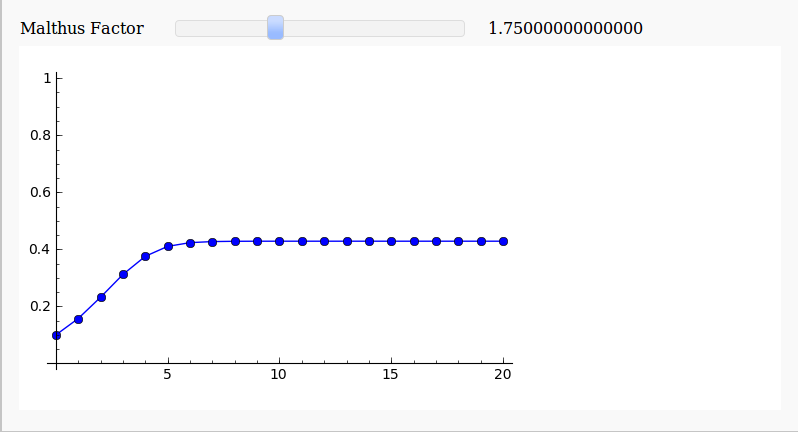
Here’s a screenshot for a Malthus Factor of 1.75

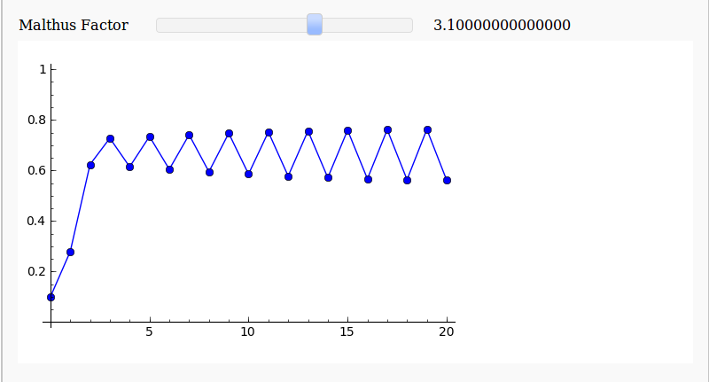
and here’s one for a Malthus Factor of 3.1

There are now so many different ways to easily make interactive mathematical demonstrations that there really is no excuse not to use them.
Update (11th December 2009)
As Harald Schilly points out, you can make a nice fractal out of this by plotting the limit points. My blogging software ruined his code when he placed it in the comments section so I reproduce it here (but he’s also uploaded it to sagenb)
var('x malthus')
step(x,malthus) = malthus * x * (1-x)
stepfast = fast_callable(step, vars=[x, malthus], domain=RDF)

def logistic(m, step):
   # filter cycles
   v = .5
   for i in range(100):
       v = stepfast(v,m)
   points = []
   for i in range(100):
       v = stepfast(v,m)
       points.append((m+step*random(),v))
   return points
points=[]
step = 0.005
for m in sxrange(2.5,4,step):
   points += logistic(m, step)
point(points,pointsize=1).show(dpi=150)


If you just plot the limit points you get a nice fractal ;)
cell 1:
var(‘x malthus’)
step(x,malthus) = malthus * x * (1-x)
stepfast = fast_callable(step, vars=[x, malthus], domain=RDF)
def logistic(m, step):
# filter cycles
v = .5
for i in range(100):
v = stepfast(v,m)
points = []
for i in range(100):
v = stepfast(v,m)
# points with horizontal jitter
points.append((m+step*random(),v))
return points
cell 2:
points=[]
step = 0.005
for m in sxrange(2.5,4,step):
points += logistic(m, step)
point(points,pointsize=1).show(dpi=150)
Ok, that’s ugly here… published on sagenb.org
http://sagenb.org/pub/1240/
You might be interested in these interacts if you haven’t seen them already:
http://wiki.sagemath.org/interact/dynsys
Cheers,
Marshall
Hi Marshall
So your logistic map interact is ‘cythonized’ – pretend I am an idiot for a while (not too much of a stretch I know)……
Cythonized means that those functions run as compiled-C right? Or put another way…very VERY fast?
Cheers,
Mike
Hi Mike,
Thanks for blogging about this. I’ve done something very similar as a lab in Calc I (not Cythonized, though, so probably slower than Marshall’s), and for pedagogical use I found it helpful to make sliders for the starting population and the step size as well. This particularly shows (as with other Euler-type approximations) that the ‘chaotic’ coefficients and behavior depend a lot on the step size, but not so much on the starting point (with certain exceptions). Of course, given your description in ‘about’, probably you won’t need it too much for teaching :) but anyway it’s fun to think about how to use these capabilities.
Best,
– kcrisman
I’ve made this (the limit-y, fractal-y) demo a million times in Mathematica a million different ways, and every time I see it I love it more :D
@Connor – a million different ways huh? Sounds interesting! Care to post a couple? ;)
@Kcrisman – I don’t teach maths but I do teach math software – often to lecturers or postgrads. I like examples such as this because they show what can be achieved with very little actual effort