Walking Randomly

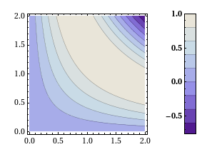
Will Robertson and I have released a new version of our colorbarplot package for Mathematica 6 and above.  Colorbarplot has only one aim and that is to allow Mathematica users to add a MATLAB-like colorbar to their graphs.  Something like this for example:

Version 0.5 is a very small upgrade from 0.4 in that it allows you to change the font style of the colorbar ticks as well as it’s label – as requested by Murat Havzalı.  Here are a couple of examples of the new functionality:

ColorbarPlot[Sin[#1 #2] &, {0, 2}, {0, 2},
 PlotType -> "Contour",
 CTicksStyle -> Bold]

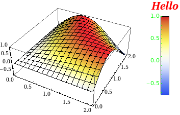
ColorbarPlot[Sin[#1 #2] &, {0, 2}, {0, 2},
 PlotType -> "3D",
 CLabel -> "Hello",
 ColorFunction -> "TemperatureMap",
 CLabelStyle -> Directive[Red, Italic, Bold, FontSize -> 20],
 CTicksStyle -> Directive[Green, FontFamily -> "Helvetica"]
 ]

Colorbarplot comes with an extensive examples file and you can download version 0.5 either from me or from Will’s github repository. We hope you find it useful and comments are welcomed.

• UPDATE 12th Novermber 2010. Update to version 0.6

So here’s a way of using Mathematica that, I have to admit, never occurred to me.

Essentially the idea is to make a big, empty graphic and then use the 2d drawing tools palette tools along with equation palettes and the ‘Evaluate in place’ menu item to produce a Mathcad-like interface. I like it!

It’s a neat trick but I highly doubt that it would be enough to lure Mathcad users away from their application of choice. Any thoughts?

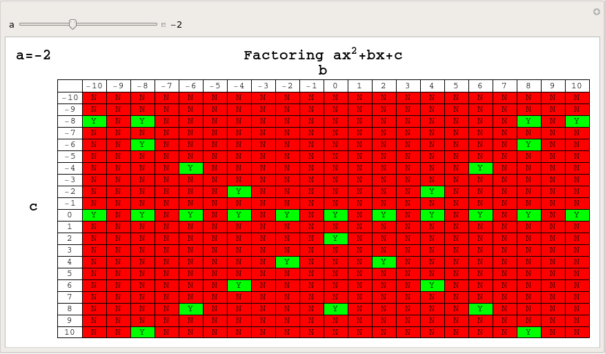
In his blog post, Factoring Schmactoring,  Sam Shah took a look at how many quadratic equations of the form x^2+bx+c = 0 (where b and c are integers) could be factored over the integers and produced a chart that was a powerful reminder of just how few of these there are.

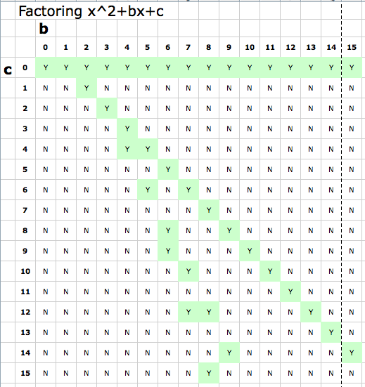
After reading his post I fired up Mathematica and set to work extending Sam’s original chart to include negative values of b and c – the result of which is shown below.  Out of 441 different quadratic equations, only 76 have integer solutions which is only 17.23%, and yet these are the only ones that succumb to the heavily drilled and killed method of factoring.

Sam and his commentators discussed the serious question of whether or not we should even be teaching factoring these days (for the record, I think we should) but my concerns were much less lofty.  I wondered if I’d make something pretty if I did a similar chart to the one above but for values of b and c ranging from -100 to 100.

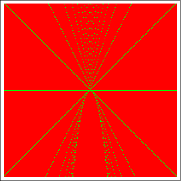
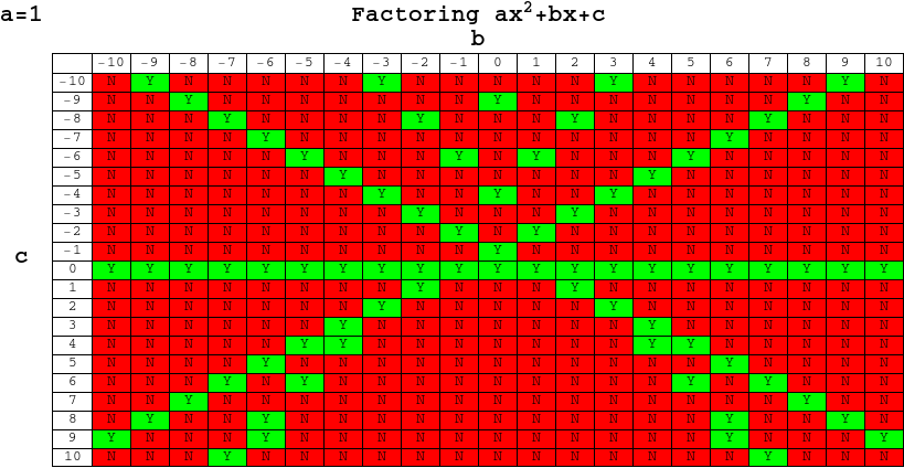
OK, so it’s not so pretty but it is possibly even more striking than the original charts – there is a LOT of red.  Next, I wondered about values of a (the x^2 coefficient) other than 1 and thought that this was the perfect situation for a Manipulate (Click on the image to download an interactive version which can be used in either Mathematica or the free Mathematica Player):

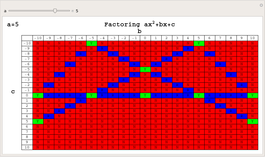
Of course, when dealing with values of a other than one, we should include the possibility of rational solutions so let’s do that and assign rational solutions to the colour blue – again click on the image below for the Mathematica-Payer compatible interactive version.

I’m not really going anywhere with this – just having a bit of fun with Mathematica but comments are welcome.

Mathematica has a large set of functions that you can use to test the properties of numbers.  For example

IntegerQ[x]

returns True if x is an integer and False if it isn’t.  Of course you are not just restricted to asking if x is an integer or not.  For example, you can ask if it is an even number

EvenQ[x]

or an odd number

OddQ[x]

Perhaps you are wondering if x is prime

PrimeQ[x]

or even if it is an algebraic integer

AlgebraicIntegerQ[x]

The observant reader will notice that all of these functions end with a capital Q and a way of remembering this is to think that you are asking a question of the variable x.  So the question ‘Is x an integer‘ becomes, in Mathematica notation, IntegerQ[x].

I am currently working on a piece of code where I need to determine whether or not a particular number belongs to the set of rationals and I assumed that a suitable function would exist in Mathematica and that it would be called RationalQ[] so I was rather surprised to see that there is no such function in Mathematica 7.

So, I’ll just have to come up with my own.  A quick search resulted in the following function definition from Bob Hanlon

RationalQ[x_] := (Head[x] === Rational)

Which almost does what I need.  It handles the following correctly

RationalQ[1/2] (gives True)

RationalQ[Sqrt[2]] (Gives False)

but I needed a version of RationalQ that also returned True when passed an integer.  After all, the integers are just a subset of the rationals.  A moments thought resulted in

RationalQ[x_] := (Head[x] === Rational || IntegerQ[x]);

Which seems to work perfectly.  So, I offer the above function for anyone who is googling for a RationalQ function and I also ask the following questions to any Mathematica gurus who might be reading this

• Is there anything wrong with the above definition?
• Why isn’t such an obvious function not included in Mathematica as standard?

One of the things I love most about blogging is the interaction with readers via the comments section.  Put simply you guys know your onions and although I (hopefully) have something useful and/or interesting to tell you, there is a heck of a lot of stuff that you could tell me.

In the comments section of one of my recent posts, Sander Huisman, did exactly that when he suggested that I shouldn’t always use Table in Mathematica when generating lists.  This was news to me – I thought that Table was the accepted and possibly the fastest way to do it in Mathematica but it seems not.  Here is a concrete example as provided by Sander.

AbsoluteTiming[Table[PrimeQ[i], {i, 0, 10000000}];]
AbsoluteTiming[PrimeQ /@ Range[0, 10000000];]

Both of these Mathematica expressions test each of the first 10000000 integers (including 0) to see if they are prime and what you end up with is a list of Booleans – {False, False, True, True, False, True, False, True, False, False} and so on. The difference is that the first expression is noticeably slower than the second.

If, like me, you struggle to remember what the punctuation operators (/. /@ etc) actually do in Mathematica then know that foo /@ bar is equivalent to Map[foo,bar] where foo is a funbction and bar is a list.

On one of my test machines, the first expression evaluated in 10.012 seconds on average whereas the second evaluated in 8.28 seconds on average (both averages are over 100 runs).

So Map is faster than Table right?

Maybe, maybe not.  Try the following examples (again provided by Sander) where we generate a list of i+2 for i between 1 and 10^7.

AbsoluteTiming[ Table[i + 2, {i, 10^7}];]
AbsoluteTiming[# + 2 & /@ Range[10^7];]

For this calculation Table did it in 0.66 seconds and /@ (or Map) did it in 0.96 seconds (both averaged over 100 runs). As Sander says ‘Sometimes it is worth looking in to the way you make a list!’.

Comments welcomed.

Take a wheel of radius 1 and set it rotating about its axis with a frequency of 1 turn per second. Attach a second wheel, of radius 1/2, to the circumference of the first and set this second wheel rotating about its axis at a frequency of 7 turns per second. Finally, attach a third wheel to the circumference of the second and set this wheel to rotate about it’s axis at a frequency of 17 turns per second.

Now, consider a point on the circumference of the third wheel. What pattern will it trace out as the three wheels rotate?  Click on the video below to find out.

I first came across this idea in a Wolfram demonstration by Daniel de Souza Carvalho.  Daniel’s demonstration focused on the fact that you could write down the equations of these curves in two different ways. If the wheels are rotating with frequencies a, b and c respectively then you can either describe the corresponding curve with a pair of parametric equations as follows:

or as a complex valued equation:

This was a nice demonstration but I wanted to see what sort of patterns I could get by changing the frequencies of the wheels. So, I downloaded Daniel’s demonstration, added some sliders and tick boxes and then uploaded the result. Wolfram Research cleaned up my code a bit and the result was published as the Wolfram Demonstration Wheels on Wheels on Wheels.

It turns out that you can get a LOT of different patterns out of this system as you can see below.

These systems were considered in the paper “Wheels on Wheels on Wheels—Surprising Symmetry,” Mathematics Magazine 69(3), 1996 pp. 185–189 by F. A. Farris. In this paper, Farris showed that the resulting curve exhibits m-fold symmetry if the three frequencies are congruent (mod m).

Can you think of any interesting variations to this system?

Update (6th July 2009): Taki has written another version of this demonstration which includes an animation of the wheels and also looked at an example with four wheels over at his blog, Mesh Mess.

Someone emailed me recently complaining that the ParallelTable function in Mathematica didn’t work.  In fact it made his code slower!  Let’s take a look at an instance where this can happen and what we can do about it. I’ll make the problem as simple as possible to allow us to better see what is going on.

Let’s say that all we want to do is generate a list of the prime numbers as quickly as possible using Mathematica.  The code to generate the first 20 million primes is very straightforward.

primelist = Table[Prime[k], {k, 1, 20000000}];

To time how long this list takes to calculate we can use the AbsoluteTime function as follows.

t = AbsoluteTime[];
primelist = Table[Prime[k], {k, 1, 20000000}];
time2 = AbsoluteTime[] - t

This took about 63 seconds on my machine. Taking a quick look at the Mathematica documentation we can see that the parallel version of Table is, obviously enough, ParallelTable. What could be simpler? So, to spread this calculation over both processors in a dual-core laptop we simply need to do the following

t = AbsoluteTime[];
primelist = ParallelTable[Prime[k], {k, 1, 20000000}];
time2 = AbsoluteTime[] - t

The result? 98 seconds!  So, it seems that the parallel version is more than 50% SLOWER! My correspondent was right – ParallelTable doesn’t seem to work at all.

Before we send a message to Wolfram Tech Support though, let’s dig a little deeper. It turns out that a single evaluation of
Prime[k] for any given k is very quick – even for high k. Prime[100000000] evaluates in a tiny fraction of a second for example (try it! – it really is astonishingly quick.)

What I suspect is happening here is that when you move to the parallel version, the kernels spend most of the time communicating with each other rather than actually calculating anything.  I think that ParallelTable does something roughly like the following.

Kernel1:Give me a k.
Master:have k=1.
Kernel2:Give me a k.
Master:have k=2
Kernel1:I’ve done k=1 and the answer is 2, give me another k
Master: have k=3
kernel2:I’ve done k=2 and the answer is 3, give me another k etc

So, the kernels spend more time talking about the work that needs to be done rather than actually doing it. Also, for various reasons, kernel1 and kernel2 might get out of sync and so the Master kernel may end up with a list out of order.  If so then it will need to reorder the lists at the end of the calculations and so that’s even more time taken.

So, my approach was to try and reduce the amount of communication between kernels to something like

Master: Kernel 1 – you go away and get me first 10 million primes. Don’t bother me until it’s done.
Master: kernel 2 – you go away and get me the second 10 million. Don’t bother me until it’s done.

The following Mathematica code does this.

t = AbsoluteTime[];
job1 = ParallelSubmit[Table[Prime[k], {k, 1, 10000000}]];
job2 = ParallelSubmit[Table[Prime[k], {k, 10000001, 20000000}]];
{a1, a2} = WaitAll[{job1, job2}];
time2 = AbsoluteTime[] - t

This works in 40 seconds compared to the original time of 62 seconds. Not a 2x speedup but not too shabby for so little extra work on our part.

The moral of the story? Make sure that your code spends more time actually doing work than it does just talking about it.

Disclaimer: I am still learning about Mathematica’s parallel tools myself so don’t take this stuff as gospel. Also, there are almost certainly more efficient ways of getting a list of primes than using the Prime[k] function. I am only using Prime[k] here because it is an example of a function that evaluates very quickly.

Up until now I have been using Wolfram Alpha as the ultimate geek toy and have been truly delighted with it but I thought it was high time I tried to consider how one might use it more seriously.  So I set myself a task.  Nothing too complicated you understand , after all I am still finding my feet with this new system, but something that may at least possibly come up in the real world.  The task I set myself was

Obtain the actual data points for the Gross Domestic Product (GDP) of the UK from 1970 to 1980 inclusive.  To allow me to import this data into pretty much every analysis program on the planet I’ll want it in a CSV file of the form

1970,GDP of UK for 1970
1971,GDP of UK for 1971
etc

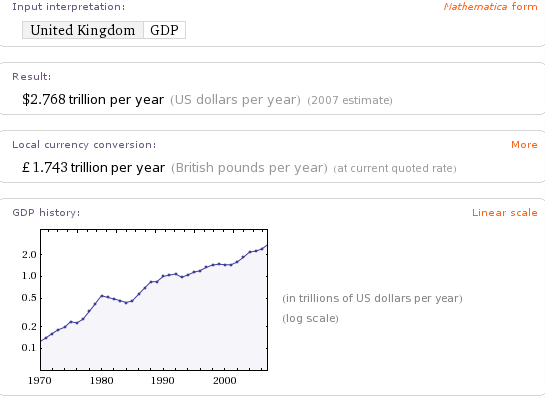
Should be easy huh?  Wolfram Alpha knows all about the GDP of the UK – if I Wolf GDP UK then I get the following output among other things).

Fabulous! The data is clearly in there but how do I get it out in the form I want? Let’s try the hopeful UK GDP from 1970 to 1980.  Alas I get the now familiar ‘Wolfram|Alpha isn’t sure what to do with your input.’ Moving on, I tried UK GDP 1970 to 1980 and UK GDP 1970-1980 but they didn’t work either.

I can get at a single datum easily enough.  UK GDP 1970 gives me 123.7 billion for example but how do I get it to give me a list?  Further experimentation showed me that I can get the GDP for any two years if I Wolf for something like (UK GDP 1970) (UK GDP 1971).

By now I feel I am getting somewhere. While playing with Wolfram Alpha (and reading the community forum) I’ve discovered that it will sometimes parse Mathematica code as well as plain English. ‘What I need‘, I thought, ‘is a piece of Mathematica code that would generate the query for me‘. So I tried

Table[“(GDP UK ” <> ToString[x] <> “)”, {x, 1970, 1980}]

but that didn’t work but then I shouldn’t be surprised because Table turns out to be one of the Mathematica functions that Wolfram Alpha doesn’t parse. Ho hum…

I tried a LOT of different inputs but the practical upshot is that the only one that worked was (UK GDP 1970) (UK GDP 1971) (UK GDP 1972) (UK GDP 1973) (UK GDP 1974) (UK GDP 1975) (UK GDP 1976) (UK GDP 1977) (UK GDP 1978) (UK GDP 1979) (UK GDP 1980).  Lord help me if I wanted three times as many data points.

For the record I can get exactly what I wanted in Mathematica 7 with the following two lines of code and I worked out how to do it with a moments thought.  Wolfram Alpha needs to be this easy!

data = Table[{x, CountryData["UK", {"GDP", x}]}, {x, 1970, 1980}];
Export["GDP.csv", data]

So, after some blood sweat and tears I had some actual numerical data but how could I export it to something useful.  Wolfram Alpha always returns results as images by default.

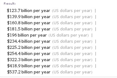
Which are not particularly useful if you want to do your own analysis.  I can also get it as copyable plaintext and for this data set it looks like this

$123.7 billion per year  (US dollars per year)  |  $139.9 billion per year  (US dollars per year)
|  $160.8 billion per year  (US dollars per year)|  $181.5 billion per year  (US dollars per year)
|  $196 billion per year  (US dollars per year)  |  $234.4 billion per year  (US dollars per year)
|  $225.2 billion per year  (US dollars per year)  |  $254.4 billion per year  (US dollars per year)
|  $322.3 billion per year  (US dollars per year)  | $418.9 billion per year  (US dollars per year)  |
  $537.2 billion per year  (US dollars per year)

Hmmm. That’s going to need some pre-processing before I can import it into Excel I think – a job for a student or a Python script I think.

Now onto the Source information. It listed it’s primary sources as ‘Wolfram Alpha Curated data 2009’ and ‘Wolfram Mathematica CountryData’ with a shed load of Secondary sources such as ‘The US CIA WorldFactbook’. I have to say that I was a little surprised at this – how is Wolfram Alpha the Primary source of this data set? They must have got it from somewhere and THAT somewhere would be the primary source (or closer to it at least) IMHO.

In all honesty, I feel that putting itself as the primary source for data such as this is a bit like a student writing an essay and under ‘references‘ simply putting ‘My head‘.

Don’t get me wrong, I am starting to love Wolfram Alpha and think it’s got amazing potential but when you love someone you always want to see them do better for themselves.  In this particular area I think that Wolfram needs to address the following

• Make it easier to get lists of data out of WA. Being able to parse Table[] might be a good start
• Allow export of tabular data in popular formats such as CSV and Excel.
• Work on the sources information a little.  Wolfram Alpha didn’t actually generate this GDP data – they must have got it from somewhere and that should be listed as primary source.

Wolfram Alpha is a constantly moving target and it is quite possible that all of these issues will be addressed in no time (if Wolfram agrees that they are issues of course) so feel free to point out if any of the inputs I have linked to give different results from those stated here.  I am also aware that I don’t know everything about this system so if I am being an idiot then feel free to point out how I should have phrased my query.  Finally, if any new functionality comes online that makes all of this trivial then I would love to know.

Comments are, as always, welcomed.

The Wolfram alpha blog has posted a set of Wolfram Alpha examples where it does some pretty complicated mathematics.  For example it can calculate the eigenvalues and eigenvectors of a 3×3 symbolic matrix – just the sort of thing you might turn to Mathematica for.

In another example it shows the result of a symbolic integral (which Mathematica can do) and it gives the steps that a human would need to do to get the same result (which Mathematica can’t do).

I know that Mathematica can do inifnitely more than one-liner calculations such as these but it makes me wonder.  Will there be less call for the new, cheap(er) home editition of Mathematica once Wolfram Alpha goes live?

Last month I (along with half of the blogging world it seems) reported on a new project from Wolfram Research called Wolfram Alpha.  At the time I didn’t know much about it but since then much more information has been available.

Rather than write more about it myself, I will simply refer you to the information I have seen.  First of all, the video below is a recording of a talk given by Stephen Wolfram about the project a couple of days ago.  Click here if you prefer to watch this directly on YouTube.

Secondly, a new blog has started up called (predictably enough) The Wolfram Alpha blog.   The first article is called The Quest for Computable Knowledge: A Longer View.

Many people are comparing Wolfram Alpha to Google which is completely wrong as far as I can tell.  It’s a bit like comparing a table of logarithms with a computer algebra system (CAS) that can calculate any logarithm you like, in any base along with the ability to plot a graph of any function that contains a logarithm.  The CAS can also differentiate, integrate, and simplify equations containing logarithms and so on.  The table of logarithms contains pre-computed data that you can search whereas the CAS can do computations based on your ‘searches’ on the fly.

Let’s take an example from the talk that Stephen gave.  Say you enter

6000C

(I assume this is what he entered, the video wasn’t so hot on showing the overhead projector connected to his laptop.  I’d give good money to get some slides right now)

Wolfram Alpha tries to tell you something useful about this input drawing from the data-sets that it has access to.  It also COMPUTES potentially useful things from these data sets.  It’s the computation part that makes it fundamentally different from google (NOTE: I said different from, not better than or a competitor to – the distinction is important in my opinion).

Wolfram Alpha will say something like ‘assuming that C is a unit and assuming that unit is Celsius then I can tell you the following about 6000C’  It will then go on to tell you various conversion factors (such as, I guess, what it would be in degrees Fahrenheit or Kelvin).  It might plot the black body spectrum at 6000 degrees C and show what colour a black-body object at that temperature would be.

All of these results will have been computed from scratch based upon various mathematical formulae and models that Wolfram Alpha has access to.  Google, on the other hand, would only show the black body spectrum at 6000C if someone had calculated it in advance and put it up on a webpage.

Of course Wolfram Alpha knows a lot more than just temperatures.  It knows about weather statistics, economic data, the human genome, properties of materials, symbolic integrals (and how to do them by hand) and loads more.

Looks like an exciting project!  I wonder how Wolfram will make money out if it (or even if it intends to)?