
Archive for the ‘mathematica’ Category
Mathematica 6.0.2 was released back on February 25th but I have only just managed to find the time to install it. I tried to install it on a brand new Dell 755 with a very fresh install of Ubuntu but near the end of the install procedure I came across the following error
“The installer was unable to check for a valid password file. Your Mathematica installation may be incomplete or corrupted.”
I had not been given the opportunity to supply it with any licensing information so it looked like there was a problem with the installer itself. Cutting a long story sort, the solution is to use apt to install the package libstdc++5 as follows
sudo apt-get install libstdc++5
This is a very common package and I guess that I have not seen this error before because libstdc++5 is automatically installed as a prerequisite for many other Ubuntu applications. Hopefully this little note will be of use to a googler or two.
Anyway…I now have 6.0.2 installed and running so expect a breakdown of the new features soon.
Next Friday will be March 14th which is celebrated by some as Pi Day since the date is 3/14 in American date format and the first three digits of Pi are 3.14 (as if I have to tell you!). One or two people have been looking for inspiration as to what to do for Pi Day in schools and I thought that it would be fun to write a Wolfram Demonstration especially for Pi Day, after all, my Valentine’s day demonstrations turned out to be quite popular.
So the question that remained to be answered was “what demonstration should I write?”
I have already written a post about making music out of the digits of Pi and discovered that a great demonstration had been written by Hector Zenil so there was no point in thinking about that.
How about Buffon’s needle? That’s a fun problem that leads to an approximation of Pi. Unfortunately for me – this is a demonstration that has already been written.
Perhaps I could do something that looked at the randomness in the digits of Pi? After all – this blog IS called walking randomly and I haven’t looked at randomness very much yet. Unfortunately I have been beaten to this one too (By Stephen Wolfram himself no less).

My next thought was to consider some series that would sum up to approximations of Pi. Again – it’s been done.

In addition to these three there are many others such as
- Consecutive Digits in the Expansion of Pi
- Pi Digits Bar Chart
- Pi Digits Pie
- Wallis’ Sieve Pi Approximation
- Graphs Of Successive Digits Of Pi, E and Phi
- Wallis Formula
That’s a lot of Pi and I have only just gotten started. All in all I am stumped – I have no idea of a demonstration I might write for Pi Day but if you can think of something then let me know and I will see what I can do :) (Oh and I will make sure that you get credit for your idea when I submit it to the project)
A couple of weeks ago I started thinking about Valentine’s day and, since I like equations that have interesting plots so much, I wondered if I could find one that had a heart-shaped graph. A quick google search came up Wolfram Research’s Heart Surface page.
The main page described a couple of heart shaped algebraic surfaces which looked nice but there were a few more on the Mathematica notebook that the page linked to. This notebook was rather old and included plots from old versions of Mathematica so on the train ride home I wrapped these equations in some Manipulate functions and sent the resulting demo to Wolfram. The result was published today on the Wolfram Demonstrations site.

Essentially all this demo does is use Mathematica’s ContourPlot3D function to plot the curves formed from the following equations and allow you to play with the results a bit.
Nordstrand

Kuska

Taubin

Trott

Each equation is named after the person who first wrote it down (to my knowledge at least). It’s a simple demo but I hope you like it.
Happy Valentine’s day.
I imagine that most of the people reading this will know what the Tangram puzzle is but just in case you are not one of them here is a quick excerpt from the Wikipedia page which says it all:
“Tangram (Chinese: 七巧板; pinyin: qī qiǎo bǎn; literally “seven boards of skill”) is a dissection puzzle. It consists of seven pieces, called tans, which fit together to form a shape of some sort. The objective is to form a specific shape with seven pieces. The shape has to contain all the pieces, which may not overlap. ”
The classical Tangram puzzle looks like this:

It is possible to make many shapes from these pieces; some of which are below (taken from tangrams.ca)

If you would like to have a go at making your own Tangram shapes then you can make your own Tangram set out of paper, buy a nice wooden one, try this java applet or use this Mathematica demonstration (written by ) using the free Mathplayer from Wolfram Research. There is even a Tangram game for the Nintendo DS
!
In the week leading up to Valentine’s day I wondered if there is a standard variation of the classical Tangram puzzle that is constructed from a heart shape and I was delighted to discover that there is. Using Enrique’s Mathematica code as a starting point I wrote a demonstration called Broken Heart Tangram and it was published on the Wolfram Demonstrations site today.

I hope you have fun with this demonstration and would love to see some of the shapes that you come up with. As always, comments are welcomed.
Other articles you may like
For my final Valentine’s day post I thought I would share a minor discovery I made while playing around with the polar equation

When n=1 the graph of this equation is a rotated cardioid which is exactly what I expected after reading the Math World page on the Heart Curve.

While playing around with the parameters I discovered that if you increase the value of n (to 10 say) then the resulting plot looks like a flower.
Very apt considering the time of year I think. If you would like to play with this equation yourself then feel free to try my very simple Wolfram Demonstration which was published today.
A little while ago I discovered that if you plot the following equation over a certain range then the result is rather surprising.

A lot of people seemed to like this post and quite a few people reproduced the graph on their website so I thought I would revisit it. To allow people to play with this equation I have written a Wolfram Demonstration which was published yesterday; a screen shot is below.
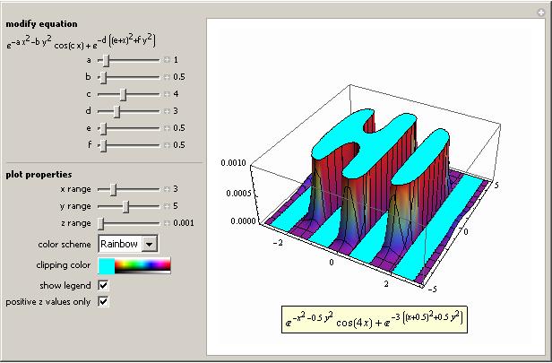
Head over to Wolfram’s site in order to download it (and the source code if you wish). Remember you do not need to have a copy of Mathematica in order to run demonstrations such as this one – the free MathPlayer will do the job nicely.
In a recent post over at 360 the author was discussing how Joe Turner (a prof of musical composition) has formed a musical composition based on the expansion of Pi in base 12 and it sounds pretty good considering the fact that it is based on a random sequence. This was picked up by another blog I discovered recently (thanks to the carnival of mathematics) where the author asked if anyone else would mind producing similar compositions based on other mathematical constants.
On the train journey home from work I thought that I might be able to get Mathematica to produce simplified versions of these sort of compositions without too much effort. So I fired up my copy of Mathematica, plugged in some headphones (I was fairly sure that my fellow commuters would not appreciate the music of Pi as much as I) and set to work. Although I knew that Mathematica had sound capabilities I had never used them before so the help browser (as usual) was indispensable.
I am going to present the rest of this post as a tutorial, with Mathematica commands in bold followed by the output in normal tyle. This is my first attempt at a tutorial in a blog post so feedback would be welcomed.
From the help browser I discovered that you can represent a note in Mathematica using SoundNote. Middle C is represented by SoundNote[0], one semi-tone above middle C is SoundNote[1] , a whole tone above Middle C is SoundNote[2] and so on. You can also use negative numbers so that SoundNote[-1] is one semi-tone below middle C for example.
So far so good but I don’t want to just represent the notes symbolically – I want to actually play them. The way to do this is by wrapping a SoundNote expression with Sound[]. So to play a middle C just evaluate
Sound[SoundNote[0]]
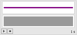
A little interface appears that looks like the graphic above and when you click the play button (represented by a triangle) you will hear a piano sample at middle C that lasts for one second.
So far so good – I have a way of playing any integer I choose but I need to be able to play a list of notes if I am going to convert Pi to music. For those of you who don’t know much about Mathematica all you need to do to create a list of ANYTHING is separate them by commas and wrap the whole thing in curly braces {} so a list the integers 1 to 5 looks like this
{1,2,3,4,5}
A list of strings looks like this
{“hello”,”world”,”these”,”are”,”strings”}
Finally, a list of three SoundNotes looks like this:
{SoundNote[3], SoundNote[1], SoundNote[4]}
Wrap this list with Sound[] to play the three notes in sequence:
Sound[{SoundNote[3], SoundNote[1], SoundNote[4]}]
So all I need now is to get the digits of Pi (or any other number I might choose) into a list of SoundNotes. If all I wanted was the decimal expansion of Pi to any number of digits I choose then I could use the N command:
N[Pi,20]
3.1415926535897932385
Since the original article asks for Pi in base twelve I could use BaseForm[number,base] to display Pi in base 12 as follows:
BaseForm[N[Pi,20],12]
3.184809493b9186645712
This is all well and good but what I actually want is a list of the digits of Pi in base 12 and so I am going to use the RealDigits command which has the syntax RealDigits[number,base,number_of_digits]. This returns a list of the digits of your number according to your specified base and number of digits. So to get a list of the first 20 digits of Pi in base 12 I do
RealDigits[Pi, 12, 20]
{{3, 1, 8, 4, 8, 0, 9, 4, 9, 3, 11, 9, 1, 8, 6, 6, 4, 5, 7, 3}, 1}
Now this result is not just a simple list but is list of lists instead. The first element is a list of the digits of Pi in base 12 and the second element is the number of digits to the left of the decimal point. I only want the first element of this list of lists – namely the list of digits of Pi. To extract elements from lists in Mathematica you use double square brackets [[ ]] so to get the 3rd element of the list {1,4,9,16,25} you would type
{1,4,9,16,25}[[3]]
9
So to get that first list from the result of RealDigits[Pi, 12, 20] we do
RealDigits[Pi, 12, 20][[1]]
{3, 1, 8, 4, 8, 0, 9, 4, 9, 3, 11, 9, 1, 8, 6, 6, 4, 5, 7, 3}
So far so good but we are not done yet – somehow I need to wrap each integer in this list with SoundNote[]. One way to do this is by using Map[]. For example I can wrap each element of the list {3,1,4} with SoundNote by doing
Map[SoundNote,{3,1,4}]
{SoundNote[3], SoundNote[1], SoundNote[4]}
Applying this knowledge to the code we have built up so far allows us to write the following
Map[SoundNote,

RealDigits[Pi, 12, 20][[1]]

]
{SoundNote[3], SoundNote[1], SoundNote[8], SoundNote[4], SoundNote[8],SoundNote[0], SoundNote[9], SoundNote[4], SoundNote[9],SoundNote[3], SoundNote[11], SoundNote[9], SoundNote[1],SoundNote[8], SoundNote[6], SoundNote[6], SoundNote[4], SoundNote[5],SoundNote[7], SoundNote[3]}
I have started to format my Mathematica commands a bit to make them more readable by using multiple lines. This is not necessary but I find that if I don’t do this then I soon start to loose track of all those square brackets and get into a horrible mess. All that I have to do now is wrap this result with Sound[] and my job is done.
Sound[

Map[SoundNote,

RealDigits[Pi, 12, 20][[1]]

]]

By modifying this group of commands you can ‘play’ any expression you like to as many decimal places as you like but there is still work to be done. For example we are stuck with only using a piano and every note has a one second duration which is far from ideal but this post is getting a bit long so I will explain how to change these in a future post if anyone is interested.
By the time my train journey was over I had produced a little ‘applet’ in Mathematica using the principles described here along with the Manipulate function. It could play Pi in any number base using any one of a range of instruments with variable note speed. I fully intended on refining it a bit and submitting it to the Wolfram Demonstrations project but when I got home and regained internet access I discovered that I had been beaten to it by someone called Hector Zenil. Hector has written a very nice demonstration called Math Songs which does exactly what I had been trying to achieve and a whole lot more. Not only can you listen to Pi but you can also listen to e, Euler’s Gamma constant, the golden ratio, the Catalan constant and a few more I haven’t even heard of.
Oh well…you can’t win them all and Hector has done a fantastic job (better than I would have done to be honest). The best thing is that you don’t even need Mathematica to play with his creation. The free (but rather large) MathPlayer will do the job nicely for you.
So, have fun with Hector’s little demonstration and I hope the mini-tutorial here was useful to someone. As always feel free to leave comments.
How good is your symbolic integral calculus? Do you think that you can do better than Mathematica? Let’s see – try and evaluate the following (there is a hint in the comments if you get stuck).

My integration skills are a little rusty but I found the solution, log(6)/4, without too much difficulty (I have picked up the habit of writing log(x) when I mean ln(x) from using computer algebra packages too much) . Let’s see how Mathematica handles the same integration. Plugging the following command into version 6
Integrate[(x^3 + 1)/(x^4 + 4*x + 1), {x, 0, 1}]
gives a solution of
(RootSum[1 + 4*#1 + #1^4 & , Log[1 – #1]/(1 + #1^3) & ] -RootSum[1 + 4*#1 + #1^4 & , Log[-#1]/(1 + #1^3) & ] +
RootSum[1 + 4*#1 + #1^4 & ,(Log[1 – #1]*#1^3)/(1 + #1^3) & ] -RootSum[1 + 4*#1 + #1^4 & , (Log[-#1]*#1^3)/(1 + #1^3) & ])/4
Ugh! Applying the FullSimplify command doesn’t help so it seems that this is the best that Mathematica can do at the moment. If you evaluate this expression numerically then it agrees with the symbolic result but I think you would agree that Mathematica has not done a very good job here.
I found this integral while looking through the changelog of the latest version of Maxima – an open source mathematics package. If you try and evaluate it in pre-5.14 versions of Maxima then it will appear to hang (actually it will return a result eventually if you leave it long enough and have enough memory but it makes the Mathematica result look positively pretty). This has been fixed in version 5.14 and now issuing the command
integrate ((x^3 + 1)/(x^4 + 4*x + 1),x,0,1);
gives the result you would expect. So what went wrong – why does such a simple integral cause problems with these powerful software packages? The answer can be found in the full Maxima bug report for this issue – I will let you read it yourself if you are interested but in a nutshell pre 5.14 versions of Maxima were attempting to use a technique from complex analysis called contour integration to evaluate this integral. Contour integration is an amazingly useful technique that can be used to evaluate all sorts of definite integrals that are very difficult to do via other methods but using it in this case was a bad idea. It is possible that Mathematica tried to evaluate the integral in the same way but since it is closed source only the developers at Wolfram know the answer to that.
So this has been fixed in Maxima and I imagine that it will only be a matter of time before it is fixed in Mathematica but until that happens why not give this integral to your students and show them that, sometimes at least, they can do calculus better than Mathematica?
Recently, someone over at comp.soft-sys.math.mathematica had a simple problem – he had a 1d array of y-values which he wanted to plot. Easy enough – if his array is in a variable called dataset all he would need to do is
Listplot[dataset]
which would create a plot of x-y values with the x values being 1,2,3….. and so on. The problem the poster had was that he wanted the x-axis to start at 100 rather than the default which is 1.
Several people, including me, tried to be helpful and posted solutions that were along the lines of ‘create an explicit set of x-values, starting at 100, do some trickery to turn the two arrays into a set of x,y pairs and plot the result’. For example you could do this with
(*Assume that the array is in a variable called dataset*)
x = Range[100, 100 + Length[dataset] - 1];
ListPlot[Transpose@{x, dataset}]
This works fine but we should have read the new version 6 documentation because (as pointed out by someone else on the forum) there is now a much easier way of doing this using the DataRange option.
ListPlot[dataset, DataRange -> {100, 100 + Length[dataset]}]
A user on comp.soft-sys.math.mathematica had a query about MD5 hashes in Mathematica that caught my attention recently. Now I was playing with MD5 in php a few days ago and one thing that I discovered was that the MD5 of a string seemed to vary depending on which program you used to generate it. For example if we use the unix command md5sum to hash the string ‘hello’ (Note the quotes are not part of the string) as follows
echo ‘hello’ | md5sum
we will get
b1946ac92492d2347c6235b4d2611184
All well and good but if we use the php md5 function to hash ‘hello’ (using the script here for example) then we get
5d41402abc4b2a76b9719d911017c592
Clearly different which was enough to annoy at least one person. It turns out that the reason for this is quite straightforward. The php function is returning the hash of the string ‘hello’ as required but the standard unix example is returning the hash of the string ‘hello\n’ where \n stands for a newline. Initially I thought this was interesting but then it hit me that the output of
echo ‘hello’
is in fact ‘hello\n’ so no one should have been surprised really. I would have quickly forgotten about this but someone was having a similar problem in Mathematica. In Mathematica strings are enclosed in double quotes so we hash the word hello as follows:
Hash[“hello”, “MD5”] // BaseForm[#, 16] &
5deaee1c1332199e5b5bc7c5e4f7f0c2
Which is completely different from our two cases above so what on earth is going on? Again, it turns out that the solution is, in fact, rather dull. It seems that Mathematica includes the enclosing double quotes when it produces the hash – which is not what I would expect at all. You can confirm this by running the string (including quotes) “hello” through the php md5 function.
I know its not exactly earth shattering stuff but I thought that I would write it up just in case someone else wondered about this stuff and was googling for it.