
Archive for the ‘programming’ Category
I was recently working on some MATLAB code with Manchester University’s David McCormick. Buried deep within this code was a function that was called many,many times…taking up a significant amount of overall run time. We managed to speed up an important part of this function by almost a factor of two (on his machine) simply by inserting two brackets….a new personal record in overall application performance improvement per number of keystrokes.
The code in question is hugely complex, but the trick we used is really very simple. Consider the following MATLAB code
>> a=rand(4000);
>> c=12.3;
>> tic;res1=c*a*a';toc
Elapsed time is 1.472930 seconds.
With the insertion of just two brackets, this runs quite a bit faster on my Ivy Bridge quad-core desktop.
>> tic;res2=c*(a*a');toc
Elapsed time is 0.907086 seconds.
So, what’s going on? Well, we think that in the first version of the code, MATLAB first calculates c*a to form a temporary matrix (let’s call it temp here) and then goes on to find temp*a’. However, in the second version, we think that MATLAB calculates a*a’ first and in doing so it takes advantage of the fact that the result of multiplying a matrix by its transpose will be symmetric which is where we get the speedup.
Another demonstration of this phenomena can be seen as follows
>> a=rand(4000);
>> b=rand(4000);
>> tic;a*a';toc
Elapsed time is 0.887524 seconds.
>> tic;a*b;toc
Elapsed time is 1.473208 seconds.
>> tic;b*b';toc
Elapsed time is 0.966085 seconds.
Note that the symmetric matrix-matrix multiplications are faster than the general, non-symmetric one.
In a recent article, Matt Asher considered the feasibility of doing statistical computations in JavaScript. In particular, he showed that the generation of 10 million normal variates can be as fast in Javascript as it is in R provided you use Google’s Chrome for the web browser. From this, one might infer that using javascript to do your Monte Carlo simulations could be a good idea.
It is worth bearing in mind, however, that we are not comparing like for like here.
The default random number generator for R uses the Mersenne Twister algorithm which is of very high quality, has a huge period and is well suited for Monte Carlo simulations. It is also the default algorithm for modern versions of MATLAB and is available in many other high quality mathematical products such as Mathematica, The NAG library, Julia and Numpy.
The algorithm used for Javascript’s math.random() function depends upon your web-browser. A little googling uncovered a document that gives details on some implementations. According to this document, Internet Explorer and Firefox both use 48 bit Linear Congruential Generator (LCG)-style generators but use different methods to set the seed. Safari on Mac OS X uses a 31 bit LCG generator and Version 8 of Chrome on Windows uses 2 calls to rand() in msvcrt.dll. So, for V8 Chrome on Windows, Math.random() is a floating point number consisting of the second rand() value, concatenated with the first rand() value, divided by 2^30.
The points I want to make here are:-
- Javascript’s math.random() uses different algorithms between browsers.
- These algorithms have relatively small periods. For example, a 48-bit LCG has a period of 2^48 compared to 2^19937-1 for Mersenne Twister.
- They have poor statistical properties. For example, the 48bit LCG implemented in Java’s java.util.Random function fails 21 of the BigCrush tests. I haven’t found any test results for JavaScript implementations but expect them to be at least as bad. I understand that Mersenne Twister fails 2 of the BigCrush tests but these are not considered to be an issue by many people.
- You can’t manually set the seed for math.random() so reproducibility is impossible.
From time to time I find myself having to write or modify windows batch files. Sometimes it might be better to use PowerShell, VBScript or Python but other times a simple batch script will do fine. As I’ve been writing these scripts, I’ve kept notes on how to do things for future reference. Here’s a summary of these notes. They were written for my own personal use and I put them here for my own convenience but if you find them useful, or have any comments or corrections, that’s great.
These notes were made for Windows 7 and may contain mistakes, please let me know if you spot any. If you use any of the information here, we agree that its not my fault if you break your Windows installation. No warranty and all that.
These notes are not meant to be a tutorial.
Comments
Comments in windows batch files start with REM. Some people use :: which is technically a label. Apparently using :: can result in faster script execution (See here and here). I’ve never checked.
REM This is a comment
:: This is a comment too...but different. Might be faster.
If statements
If "%foo%"=="bar" (
REM Do stuff
REM Do more stuff
)
else (
REM Do different stuff
)
Check for existence of file
if exist {insert file name here} (
    rem file exists
) else (
    rem file doesn't exist
)
Or on a single line (if only a single action needs to occur):
if exist {insert file name here} {action}
for example, the following opens notepad for autoexec.bat, if the file exists:
if exist c:\autoexec.bat notepad c:\autoexec.bat
Echoing and piping output
To get a newline in echoed output, chain commands together with &&
echo hello && echo world
gives
hello
world
To pipe output to a file use > or >> The construct 2>&1 ensures that you get both standard output and standard error in your file
REM > Clobbers log.txt, overwriting anything you already have in it
"C:\SomeProgram.exe" > C:\log.txt 2>&1

REM >> concatenates output of SomeProgram.exe to log.txt
"C:\SomeProgram.exe" >> C:\log.txt 2>&1
Environment Variables
set and setx
- set – sets variable immediately in the current context only. So, variable will be lost when you close cmd.exe.
- setx – sets variable permanently but won’t be valid until you start a new context (i.e. open a new cmd.exe)
List all environment variables defined in current session using the set command
set
To check if the environment variable FOO is defined
if defined FOO (
 echo "FOO is defined and is set to %FOO%"
)
To permanently set the system windows environment variable FOO, use setx /m
setx FOO /m "someValue"
To permanently unset the windows environment variable FOO, set it to an empty value
setx FOO ""
A reboot may be necessary. Strictly speaking this does not remove the variable since it will still be in the registry and will still be visible from Control Panel->System->Advanced System Settings->Environment variables. However, the variable will not be listed when you perform a set command and defined FOO will return false. To remove all trace of the variable, delete it from the registry.
Environment variables in the registry
On Windows 7:
- System environment variables are at HKEY_LOCAL_MACHINE\SYSTEM\CurrentControlSet\Control\Session Manager\Environment
- User environment variables are at HKEY_CURRENT_USER\Environment
If you change environment variables using the registry, you will need to reboot for them to take effect.
Pausing
This command will pause for 10 seconds
TIMEOUT /T 10
Killing an application
This command will kill the notepad.exe window with the title Readme.txt
taskkill /f /im notepad.exe /fi "WINDOWTITLE eq Readme.txt"
Time stamping
The variable %time% expands to the current time which leads you to do something like the following to create time stamps between the execution of commands.
echo %time%
timeout /t 1
echo %time%
This works fine unless your code is in a block (i.e. surrounded by brackets), as it might be if it is part of an if-statement for example:
(
echo %time%
timeout /t 1
echo %time%
)
If you do this, the echoed time will be identical in both cases because the %time% entries get parsed at the beginning of the code block. This is almost certainly not what you want.
Setlocal EnableDelayedExpansion
(
echo !time!
timeout /t 1
echo !time!
)
Now we get the type of behaviour we expect.
Where is this script?
Sometimes your script will need to know where it is. Say test.bat is at C:\Users\mike\Desktop\test.bat and contains the following
set whereAmI=%~dp0
When you run test.bat, the variable whereAmI will contain C:\Users\mike\Desktop\
Details on %dp0 can be found at StackOverflow.
Variable substrings
This came from StackOverflow’s Hidden features of Windows batch files which is a great resource. They’ve tightened up on what constitutes a ‘valid question’ these days and so great Q+A such as this won’t be appearing there in future.
> set str=0123456789
> echo %str:~0,5%
01234
> echo %str:~-5,5%
56789
> echo %str:~3,-3%
3456
In a recent blog post, I demonstrated how to use the MATLAB 2012a Symbolic Toolbox to perform Variable precision QR decomposition in MATLAB. The result was a function called vpa_qr which did the necessary work.
>> a=vpa([2 1 3;-1 0 7; 0 -1 -1]);
>> [Q R]=vpa_qr(a);
I’ve suppressed the output because it’s so large but it definitely works. When I triumphantly presented this function to the user who requested it he was almost completely happy. What he really wanted, however, was for this to work:
>> a=vpa([2 1 3;-1 0 7; 0 -1 -1]);
>> [Q R]=qr(a);
In other words he wants to override the qr function such that it accepts variable precision types. MATLAB 2012a does not allow this:
>> a=vpa([2 1 3;-1 0 7; 0 -1 -1]);
>> [Q R]=qr(a)
Undefined function 'qr' for input arguments of type 'sym'.
I put something together that did the job for him but felt that it was unsatisfactory. So, I sent my code to The MathWorks and asked them if what I had done was sensible and if there were any better options. A MathWorks engineer called Hugo Carr sent me such a great, detailed reply that I asked if I could write it up as a blog post. Here is the result:
Approach 1: Define a new qr function, with a different name (such as vpa_qr). This is probably the safest and simplest option and was the method I used in the original blog post.
- Pros: The new function will not interfere with your MATLAB namespace
- Cons: MATLAB will only use this function if you explicitly define that you wish to use it in a given function. You would have to find all prior references to the qr algorithm and make a decision about which to use.
Approach 2: Define a new qr function and use the ‘isa’ function to catch instances of ‘sym’. This is the approach I took in the code I sent to The MathWorks.
function varargout = qr( varargin )

if nargin == 1 && isa( varargin{1}, 'sym' )
    [varargout{1:nargout}] = vpa_qr( varargin{:} );
else
    [varargout{1:nargout}] = builtin( 'qr', varargin{:} );
end
- Pros: qr will always select the correct code when executed on sym objects
- Cons: This code only works for shadowing built-ins and will produce a warning reminding you of this fact. If you wish to extend this pattern for other class types, you’ll require a switch statement (or nested if-then-else block), which could lead to a complex comparison each time qr is invoked (and subsequent performance hit). Note that switch statements in conjunction with calls to ‘isa’ are usually indicators that an object oriented approach is a better way forward.
Approach 3: The MathWorks do not recommend that you modify your MATLAB install. However for completeness, it is possible to add a new ‘method’ to the sym class by dropping your function into the sym class folder. For MATLAB 2012a on Windows, this folder is at
C:\Program Files\MATLAB\R2012a\toolbox\symbolic\symbolic\@sym
For the sake of illustration, here is a simplified implementation. Call it qr.m
function result = qr( this )
  result = feval(symengine,'linalg::factorQR', this);
end
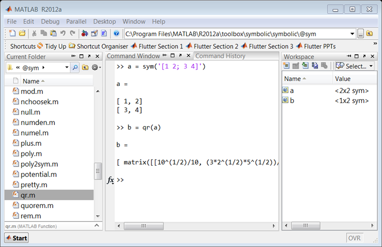
Pros: Functions saved to a class folder take precedence over built in functionality, which means that MATLAB will always use your qr method for sym objects.
Cons: If you share code which uses this functionality, it won’t run on someone’s computer unless they update their sym class folder with your qr code. Additionally, if a new method is added to a class it may shadow the behaviour of other MATLAB functionality and lead to unexpected behaviour in Symbolic Toolbox.
Approach 4: For more of an object-oriented approach it is possible to sub-class the sym class, and add a new qr method.
classdef mySym < sym

    methods
        function this = mySym(arg)
            this = this@sym(arg);
        end

        function result = qr( this )
            result = feval(symengine,'linalg::factorQR', this);
        end
    end

end
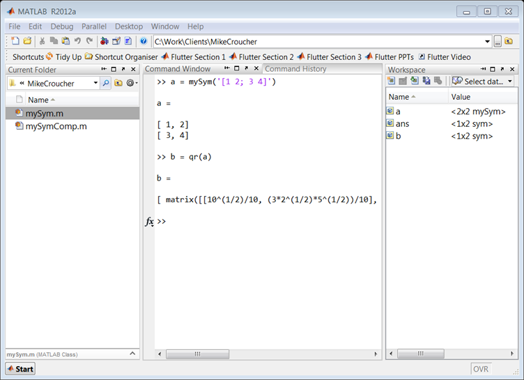
Pros: Your change can be shipped with your code and it will work on a client’s computer without having to change the sym class.
Cons: When calling superclass methods on your mySym objects (such as sin(mySym1)), the result will be returned as the superclass unless you explicitly redefine the method to return the subclass.
N.B. There is a lot of literature which discusses why inheritance (subclassing) to augment a class’s behaviour is a bad idea. For example, if Symbolic Toolbox developers decide to add their own qr method to the sym API, overriding that function with your own code could break the system. You would need to update your subclass every time the superclass is updated. This violates encapsulation, as the subclass implementation depends on the superclass. You can avoid problems like these by using composition instead of inheritance.
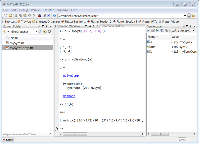
Approach 5: You can create a new sym class by using composition, but it takes a little longer than the other approaches. Essentially, this involves creating a wrapper which provides the functionality of the original class, as well as any new functions you are interested in.
classdef mySymComp

    properties
        SymProp
    end

    methods
        function this = mySymComp(symInput)
            this.SymProp = symInput;
        end

        function result = qr( this )
            result = feval(symengine,'linalg::factorQR', this.SymProp);
        end
    end

end
Note that in this example we did not add any of the original sym functions to the mySymComp class, however this can be done for as many as you like. For example, I might like to use the sin method from the original sym class, so I can just delegate to the methods of the sym object that I passed in during construction:
classdef mySymComp

    properties
        SymProp
    end

    methods
        function this = mySymComp(symInput)
            this.SymProp = symInput;
        end

        function result = qr( this )
            result = feval(symengine,'linalg::factorQR', this.SymProp);
        end

        function G = sin(this)
            G = mySymComp(sin(this.SymProp));
        end
    end

end
Pros: The change is totally encapsulated, and cannot be broken save for a significant change to the sym api (for example, the MathWorks adding a qr method to sym would not break your code).
Cons: The wrapper can be time consuming to write, and the resulting object is not a ‘sym’, meaning that if you pass a mySymComp object ‘a’ into the following code:
isa(a, 'sym')
MATLAB will return ‘false’ by default.
R has a citation() command that recommends how to cite the use of R in your publications, information that is also included in R’s Frequently Asked Questions document.
To cite R in publications use:

  R Core Team (2012). R: A language and environment for
  statistical computing. R Foundation for Statistical
  Computing, Vienna, Austria. ISBN 3-900051-07-0, URL
  http://www.R-project.org/.

A BibTeX entry for LaTeX users is

  @Manual{,
    title = {R: A Language and Environment for Statistical Computing},
    author = {{R Core Team}},
    organization = {R Foundation for Statistical Computing},
    address = {Vienna, Austria},
    year = {2012},
    note = {{ISBN} 3-900051-07-0},
    url = {http://www.R-project.org/},
  }

We have invested a lot of time and effort in creating R, please
cite it when using it for data analysis. See also
‘citation("pkgname")’ for citing R packages
This led me to wonder how often people cite the software they use. For example, if you publish the results of a simulation written in MATLAB do you cite MATLAB in any way? How about if you used Origin or Excel to produce a curve fit, would you cite that? Would you cite your plotting software, numerical libraries or even compiler?
The software sustainability institute (SSI), of which I recently became a fellow, has guidelines on how to cite software.
The Numerical Algorithms Group (NAG) are principally known for their numerical library but they also offer products such as a MATLAB toolbox and a Fortran compiler. My employer, The University of Manchester, has a full site license for most of NAG’s stuff where it is heavily used by both our students and researchers.
While at a recent software conference, I saw a talk by NAG’s David Sayers where he demonstrated some of the features of the NAG Fortran Compiler. During this talk he showed some examples of broken Fortran and asked us if we could spot how they were broken without compiler assistance. I enjoyed the talk and so asked David if he would mind writing a guest blog post on the subject for WalkingRandomly. He duly obliged.
This is a guest blog post by David Sayers of NAG.
What do you want from your Fortran compiler? Some people ask for extra (non-standard) features, others require very fast execution speed. The very latest extensions to the Fortran language appeal to those who like to be up to date with their code.
I suspect that very few would put enforcement of the Fortran standard at the top of their list, yet this essential if problems are to be avoided in the future. Code written specifically for one compiler is unlikely to work when computers change, or may contain errors that appear only intermittently. Without access to at least one good checking compiler, the developer or support desk will be lacking a valuable tool in the fight against faulty code.
The NAG Fortran compiler is such a tool. It is used extensively by NAG’s own staff to validate their library code and to answer user-support queries involving user’s Fortran programs. It is available on Windows, where it has its own IDE called Fortran Builder, and on Unix platforms and Mac OS X.
Windows users also have the benefit of some Fortran Tools bundled in to the IDE. Particularly nice is the Fortran polisher which tidies up the presentation of your source files according to user-specified preferences.
The compiler includes most Fortran 2003 features, very many Fortran 2008 features and the most commonly used features of OpenMP 3.0 are supported.
The principal developer of the compiler is Malcolm Cohen, co-author of the book, Modern Fortran Explained along with Michael Metcalf and John Reid. Malcolm has been a member of the international working group on Fortran, ISO/IEC JTC1/SC22/WG5, since 1988, and the USA technical subcommittee on Fortran, J3, since 1994. He has been head of the J3 /DATA subgroup since 1998 and was responsible for the design and development of the object-oriented features in Fortran 2003. Since 2005 he has been Project Editor for the ISO/IEC Fortran standard, which has continued its evolution with the publication of the Fortran 2008 standard in 2010.
Of all people Malcolm Cohen should know Fortran and the way the standard should be enforced!
His compiler reflects that knowledge and is designed to assist the programmer to detect how programs might be faulty due to a departure from the Fortran standard or prone to trigger a run time error. In either case the diagnostics of produced by the compiler are clear and helpful and can save the developer many hours of laborious bug-tracing. Here are some particularly simple examples of faulty programs. See if you can spot the mistakes, and think how difficult these might be to detect in programs that may be thousands of times longer:
Example 1
    Program test
      Real, Pointer :: x(:, :)

      Call make_dangle
      x(10, 10) = 0
    Contains
      Subroutine make_dangle
        Real, Target :: y(100, 200)

        x => y
      End Subroutine make_dangle
    End Program test
Example 2
Program dangle2
Real,Pointer :: x(:),y(:)
Allocate(x(100))
y => x
Deallocate(x)
y = 3
End
Example 3
      program more
      integer n, i
      real r, s
      equivalence (n,r)
      i=3
      r=2.5
      i=n*n
      write(6,900) i, r
900  format(' i = ', i5, '   r = ', f10.4)
      stop 'ok'
      end
Example 4
      program trouble1
      integer n
      parameter (n=11)
      integer iarray(n)
      integer i
      do 10 i=1,10
        iarray(i) = i
10   continue
      write(6,900) iarray
900  format(' iarray = ',11i5)
      stop 'ok'
      end
And finally if this is all too easy …
Example 5
!   E04UCA Example Program Text
!   Mark 23 Release. NAG Copyright 2011.

    MODULE e04ucae_mod

!      E04UCA Example Program Module:
!             Parameters and User-defined Routines

!      .. Use Statements ..
       USE nag_library, ONLY : nag_wp
!      .. Implicit None Statement ..
       IMPLICIT NONE
!      .. Parameters ..
       REAL (KIND=nag_wp), PARAMETER       :: one = 1.0_nag_wp
       REAL (KIND=nag_wp), PARAMETER       :: zero = 0.0_nag_wp
       INTEGER, PARAMETER                  :: inc1 = 1, lcwsav = 1,            &
                                              liwsav = 610, llwsav = 120,      &
                                              lrwsav = 475, nin = 5, nout = 6
    CONTAINS
       SUBROUTINE objfun(mode,n,x,objf,objgrd,nstate,iuser,ruser)
!         Routine to evaluate objective function and its 1st derivatives.

!         .. Implicit None Statement ..
          IMPLICIT NONE
!         .. Scalar Arguments ..
          REAL (KIND=nag_wp), INTENT (OUT)    :: objf
          INTEGER, INTENT (INOUT)             :: mode
          INTEGER, INTENT (IN)                :: n, nstate
!         .. Array Arguments ..
          REAL (KIND=nag_wp), INTENT (INOUT)  :: objgrd(n), ruser(*)
          REAL (KIND=nag_wp), INTENT (IN)     :: x(n)
          INTEGER, INTENT (INOUT)             :: iuser(*)
!         .. Executable Statements ..
          IF (mode==0 .OR. mode==2) THEN
             objf = x(1)*x(4)*(x(1)+x(2)+x(3)) + x(3)
          END IF

          IF (mode==1 .OR. mode==2) THEN
             objgrd(1) = x(4)*(x(1)+x(1)+x(2)+x(3))
             objgrd(2) = x(1)*x(4)
             objgrd(3) = x(1)*x(4) + one
             objgrd(4) = x(1)*(x(1)+x(2)+x(3))
          END IF

          RETURN

       END SUBROUTINE objfun
       SUBROUTINE confun(mode,ncnln,n,ldcj,needc,x,c,cjac,nstate,iuser,ruser)
!         Routine to evaluate the nonlinear constraints and their 1st
!         derivatives.

!         .. Implicit None Statement ..
          IMPLICIT NONE
!         .. Scalar Arguments ..
          INTEGER, INTENT (IN)                :: ldcj, n, ncnln, nstate
          INTEGER, INTENT (INOUT)             :: mode
!         .. Array Arguments ..
          REAL (KIND=nag_wp), INTENT (OUT)    :: c(ncnln)
          REAL (KIND=nag_wp), INTENT (INOUT)  :: cjac(ldcj,n), ruser(*)
          REAL (KIND=nag_wp), INTENT (IN)     :: x(n)
          INTEGER, INTENT (INOUT)             :: iuser(*)
          INTEGER, INTENT (IN)                :: needc(ncnln)
!         .. Executable Statements ..
          IF (nstate==1) THEN

!            First call to CONFUN.  Set all Jacobian elements to zero.
!            Note that this will only work when 'Derivative Level = 3'
!            (the default; see Section 11.2).

             cjac(1:ncnln,1:n) = zero
          END IF

          IF (needc(1)>0) THEN

             IF (mode==0 .OR. mode==2) THEN
                c(1) = x(1)**2 + x(2)**2 + x(3)**2 + x(4)**2
             END IF

             IF (mode==1 .OR. mode==2) THEN
                cjac(1,1) = x(1) + x(1)
                cjac(1,2) = x(2) + x(2)
                cjac(1,3) = x(3) + x(3)
                cjac(1,4) = x(4) + x(4)
             END IF

          END IF

          IF (needc(2)>0) THEN

             IF (mode==0 .OR. mode==2) THEN
                c(2) = x(1)*x(2)*x(3)*x(4)
             END IF

             IF (mode==1 .OR. mode==2) THEN
                cjac(2,1) = x(2)*x(3)*x(4)
                cjac(2,2) = x(1)*x(3)*x(4)
                cjac(2,3) = x(1)*x(2)*x(4)
                cjac(2,4) = x(1)*x(2)*x(3)
             END IF

          END IF

          RETURN

       END SUBROUTINE confun
    END MODULE e04ucae_mod
    PROGRAM e04ucae

!      E04UCA Example Main Program

!      .. Use Statements ..
       USE nag_library, ONLY : dgemv, e04uca, e04wbf, nag_wp
       USE e04ucae_mod, ONLY : confun, inc1, lcwsav, liwsav, llwsav, lrwsav,   &
                               nin, nout, objfun, one, zero
!      .. Implicit None Statement ..
!       IMPLICIT NONE
!      .. Local Scalars ..
      ! REAL (KIND=nag_wp)                  :: objf
       INTEGER                             :: i, ifail, iter, j, lda, ldcj,    &
                                              ldr, liwork, lwork, n, nclin,    &
                                              ncnln, sda, sdcjac
!      .. Local Arrays ..
       REAL (KIND=nag_wp), ALLOCATABLE     :: a(:,:), bl(:), bu(:), c(:),      &
                                              cjac(:,:), clamda(:), objgrd(:), &
                                              r(:,:), work(:), x(:)
       REAL (KIND=nag_wp)                  :: ruser(1), rwsav(lrwsav)
       INTEGER, ALLOCATABLE                :: istate(:), iwork(:)
       INTEGER                             :: iuser(1), iwsav(liwsav)
       LOGICAL                             :: lwsav(llwsav)
       CHARACTER (80)                      :: cwsav(lcwsav)
!      .. Intrinsic Functions ..
       INTRINSIC                              max
!      .. Executable Statements ..
       WRITE (nout,*) 'E04UCA Example Program Results'

!      Skip heading in data file
       READ (nin,*)

       READ (nin,*) n, nclin, ncnln
       liwork = 3*n + nclin + 2*ncnln
       lda = max(1,nclin)

       IF (nclin>0) THEN
          sda = n
       ELSE
          sda = 1
       END IF

       ldcj = max(1,ncnln)

       IF (ncnln>0) THEN
          sdcjac = n
       ELSE
          sdcjac = 1
       END IF

       ldr = n

       IF (ncnln==0 .AND. nclin>0) THEN
          lwork = 2*n**2 + 20*n + 11*nclin
       ELSE IF (ncnln>0 .AND. nclin>=0) THEN
          lwork = 2*n**2 + n*nclin + 2*n*ncnln + 20*n + 11*nclin + 21*ncnln
       ELSE
          lwork = 20*n
       END IF

       ALLOCATE (istate(n+nclin+ncnln),iwork(liwork),a(lda,sda), &
          bl(n+nclin+ncnln),bu(n+nclin+ncnln),c(max(1, &
          ncnln)),cjac(ldcj,sdcjac),clamda(n+nclin+ncnln),objgrd(n),r(ldr,n), &
          x(n),work(lwork))

       IF (nclin>0) THEN
          READ (nin,*) (a(i,1:sda),i=1,nclin)
       END IF

       READ (nin,*) bl(1:(n+nclin+ncnln))
       READ (nin,*) bu(1:(n+nclin+ncnln))
       READ (nin,*) x(1:n)

!      Initialise E04UCA

       ifail = 0
       CALL e04wbf('E04UCA',cwsav,lcwsav,lwsav,llwsav,iwsav,liwsav,rwsav, &
          lrwsav,ifail)

!      Solve the problem

       ifail = -1
       CALL e04uca(n,nclin,ncnln,lda,ldcj,ldr,a,bl,bu,confun,objfun,iter, &
          istate,c,cjac,clamda,objf,objgrd,r,x,iwork,liwork,work,lwork,iuser, &
          ruser,lwsav,iwsav,rwsav,ifail)

       SELECT CASE (ifail)
       CASE (0:6,8)
          WRITE (nout,*)
          WRITE (nout,99999)
          WRITE (nout,*)

          DO i = 1, n
             WRITE (nout,99998) i, istate(i), x(i), clamda(i)
          END DO

          IF (nclin>0) THEN

!            A*x --> work.
!            The NAG name equivalent of dgemv is f06paf
             CALL dgemv('N',nclin,n,one,a,lda,x,inc1,zero,work,inc1)

             WRITE (nout,*)
             WRITE (nout,*)
             WRITE (nout,99997)
             WRITE (nout,*)

             DO i = n + 1, n + nclin
                j = i - n
                WRITE (nout,99996) j, istate(i), work(j), clamda(i)
             END DO

          END IF

          IF (ncnln>0) THEN
             WRITE (nout,*)
             WRITE (nout,*)
             WRITE (nout,99995)
             WRITE (nout,*)

             DO i = n + nclin + 1, n + nclin + ncnln
                j = i - n - nclin
                WRITE (nout,99994) j, istate(i), c(j), clamda(i)
             END DO

          END IF

          WRITE (nout,*)
          WRITE (nout,*)
          WRITE (nout,99993) objf
       END SELECT

99999  FORMAT (1X,'Varbl',2X,'Istate',3X,'Value',9X,'Lagr Mult')
99998  FORMAT (1X,'V',2(1X,I3),4X,1P,G14.6,2X,1P,G12.4)
99997  FORMAT (1X,'L Con',2X,'Istate',3X,'Value',9X,'Lagr Mult')
99996  FORMAT (1X,'L',2(1X,I3),4X,1P,G14.6,2X,1P,G12.4)
99995  FORMAT (1X,'N Con',2X,'Istate',3X,'Value',9X,'Lagr Mult')
99994  FORMAT (1X,'N',2(1X,I3),4X,1P,G14.6,2X,1P,G12.4)
99993  FORMAT (1X,'Final objective value = ',1P,G15.7)
    END PROGRAM e04ucae
Answers to this particular New Year quiz will be posted in a future blog post.
xkcd is a popular webcomic that sometimes includes hand drawn graphs in a distinctive style. Here’s a typical example

In a recent Mathematica StackExchange question, someone asked how such graphs could be automatically produced in Mathematica and code was quickly whipped up by the community. Since then, various individuals and communities have developed code to do the same thing in a range of languages. Here’s the list of examples I’ve found so far
- xkcd style graphs in Mathematica. There is also a Wolfram blog post on this subject.
- xkcd style graphs in R. A follow up blog post at vistat.
- xkcd style graphs in LaTeX
- xkcd style graphs in Python using matplotlib
- xkcd style graphs in MATLAB. There is now some code on the File Exchange that does this with your own plots.
- xkcd style graphs in javascript using D3
- xkcd style graphs in Euler
- xkcd style graphs in Fortran
Any I’ve missed?
I recently installed the 64bit version of the Intel C++ Composer XE 2013 on a Windows 7 desktop alongside Visual Studio 2010. Here are the steps I went through to compile a simple piece of code using the Intel Compiler from within Visual Studio.
- From the Windows Start Menu click on Intel Parallel Studio XE 2013->Parallel Studio XE 2013 with VS2010

- Open a new project within Visual Studio: File->New Project
- In the New Project window, in the Installed Templates pane, select Visual C++ and click on Win32 Console Application. Give your project a name. In this example, I have called my project ‘helloworld’. Click on OK.

- When the Win32 Application Wizard starts, accept all of the default settings and click Finish.
- An example source file will pop up called helloworld.cpp. Modify the source code so that it reads as follows
#include "stdafx.h"
#include<iostream>
using namespace std;

int _tmain(int argc, _TCHAR* argv[])
{
	cout << "Hello World";
        cin.get();
	return 0;
}
We now need to target a 64bit platform as follows:
- Click on Project->helloworld Properties->Configuration Properties and click on Configuration Manager.

- The drop down menu under Active Solution Platform will say Win32. Click on this and then click on New.

- In the New Solution Platform window choose x64 and click on OK.

- Close the Configuration Manager and to return to the helloworld Property Pages window.
- At the helloworld Property Pages window click on C/C++ and ensure that Suppress Startup Banner is set to No and click OK.

- Click on Project->Intel Composer XE 2013->Use Intel C++ followed by OK. This switches from the Visual Studio Compiler to the Intel C++ compiler.
- Finally, build the project by clicking on Build->Build Solution. Somewhere near the top of the output window you should see
1> Intel(R) C++ Intel(R) 64 Compiler XE for applications running on Intel(R) 64,
Version 13.0.1.119 Build 20121008
1> Copyright (C) 1985-2012 Intel Corporation. All rights reserved.
This demonstrates that we really are using the Intel Compiler to do the compilation.
- Once compilation has completed you can run the application by pressing F5. It should open a console window that will disappear when you press Enter.

Intel have finally released the Xeon Phi – an accelerator card based on 60 or so customised Intel cores to give around a Teraflop of double precision performance. That’s comparable to the latest cards from NVIDIA (1.3 Teraflops according to http://www.theregister.co.uk/2012/11/12/nvidia_tesla_k20_k20x_gpu_coprocessors/) but with one key difference—you don’t need to learn any new languages or technologies to take advantage of it (although you can do so if you wish)!
The Xeon Phi uses good, old fashioned High Performance Computing technologies that we’ve been using for years such as OpenMP and MPI. There’s no need to completely recode your algorithms in CUDA or OpenCL to get a performance boost…just a sprinkling of OpenMP pragmas might be enough in many cases. Obviously it will take quite a bit of work to squeeze every last drop of performance out of the thing but this might just be the realisation of ‘personal supercomputer’ we’ve all been waiting for.
Here are some links I’ve found so far — would love to see what everyone else has come up with. I’ll update as I find more
- http://www.theregister.co.uk/2012/11/12/intel_xeon_phi_coprocessor_launch/ (Includes pricing and some benchmarks)
- http://www.streamcomputing.eu/blog/2012-11-12/intels-answer-to-amd-and-nvidia-the-xeon-phi-5110p/ (lots of details, programming models and comparisons with GPUs)
- http://software.intel.com/en-us/blogs/2012/11/12/introducing-opencl-12-for-intel-xeon-phi-coprocessor (Intel’s OpenCL works on Xeon Phi)
- http://www.hpcwire.com/hpcwire/2012-11-12/nag_delivers_numerical_software_to_xeon_phi.html (My favourite numerical library has already been ported to the Phi)
I also note that the Xeon Phi uses AVX extensions but with a wider vector width of 512 bytes so if you’ve been taking advantage of that technology in your code (using one of these techniques perhaps) you’ll reap the benefits there too.
I, for one, am very excited and can’t wait to get my hands on one! Thoughts, comments and links gratefully received!
Of Mathematica and memory
A Mathematica user recently contacted me to report a suspected memory leak, wondering if it was a known issue before escalating it any further. At the beginning of his Mathematica notebook he had the following command
Clear[Evaluate[Context[] <> "*"]]
This command clears all the definitions for symbols in the current context and so the user expected it to release all used memory back to the system. However, every time he re-evaluated his notebook, the amount of memory used by Mathematica increased. If he did this enough times, Mathematica used all available memory.
Looks like a memory leak, smells like a memory leak but it isn’t!
What’s happening?
The culprit is the fact that Mathematica stores an evaluation history. This allows you to recall the output of the 10th evaluation (say) with the command
%10
As my colleague ran and re-ran his notebook, over and over again, this history grew without bound eating up all of his memory and causing what looked like a memory leak.
Limiting the size of the history
The way to fix this issue is simply to limit the length of the output history. Personally, I rarely need more than the most recently evaluated output so I suggested that we limit it to one.
$HistoryLength = 1;
This fixed the problem for him. No matter how many times he re-ran his notebook, the memory usage remained roughly constant. However, we observed (in windows at least) that if the Mathematica session was using vast amounts of memory due to history, executing the above command did not release it. So, you can use this trick to prevent the history from eating all of your memory but it doesn’t appear to fix things after the event…to do that requires a little more work. The easiest way, however, is to kill the kernel and start again.
Links
- Memory Management in Mathematica
- Mathematica Session History
- ClearSystemCache[] – The system cache is another area of Mathematica that can use up some memory.