Walking Randomly

A recent trend on Facebook is to create a wordcloud of all of your posts using an external service. I chose not to use it because I tend to use Facebook for personal interactions among close friends and I didn’t want to send all of my data to another external company.

Twitter is a different matter, however! All of the data is open and it’s very easy to write a computer program to generate Twitter world clouds without the need for an external service.

I wrote a simple script in R that generates a wordcloud from the most recent 3200 tweets and outputs the top 200 words (get the code on github). The script removes many of the uninteresting words such as the, of, and that would otherwise dominate the cloud. These stopwords come from the Top100Words list of the R package qdap but I also added a few more such as ‘just’ and ‘me’ that I seem to use a lot.

This is the current wordcloud for my twitter account, walkingrandomly. Click on the image to see a bigger version. My main interests are very clear – Python programming, research software, data and anything that’s new!

Once I had seen my wordcloud, I wondered how things would look for other twitter users who I pay a lot of attention to. This is how it looks for Manchester University’s Nick Higham. Clearly he’s big on SIAM, Manchester, and Matrix Analysis!

I then looked at my manager at Sheffield University, Neil Lawrence. Neil finds data and the city of Sheffield very important and also writes about workshops, science, blog posts and machine learning a lot.

The R code that generated these wordclouds is available on github but it won’t work out of the box. You’ll need to register with twitter for app development (It’s free and fairly straightforward) and get various access keys before you can use the code.

• Get the code at github

It is possible to write quick, interactive demonstrations in a variety of languages these days. Functions such as Mathematica’s Manipulate, Sage Math’s interact and IPython’s interact allow programmers to write functional graphical user interfaces with just a few lines of code.

Earlier this week, I hosted a session in the Faculty of Engineering at The University of Sheffield where Maplesoft showed us, among other things, their version of this technology. This blog post is an extension of my notes from this part of the session.

• The Maple Worksheet for this blog post is available on github.

The series command expands a function as a power series around a point. For example, let’s expand sin(x) as a power series around the point x=0.

series(sin(x), x = 0, 10)

If we try to plot this, we get an error message

plot(series(sin(x), x = 0, 10), x = -2*Pi .. 2*Pi, y = -3 .. 3)

Warning, unable to evaluate the function to numeric values in the region; see the plotting command's help page to ensure the calling sequence is correct

This is because the output of the series command is a series data structure — something that the plot function cannot handle. We can, however, convert this to a polynomial which is something that the plot function can handle

convert(series(sin(x), x = 0, 10), polynom)

Wrapping the above with plot gives:

plot(convert(series(sin(x), x = 0, 10), polynom), x = -2*Pi .. 2*Pi, y = -3 .. 3);

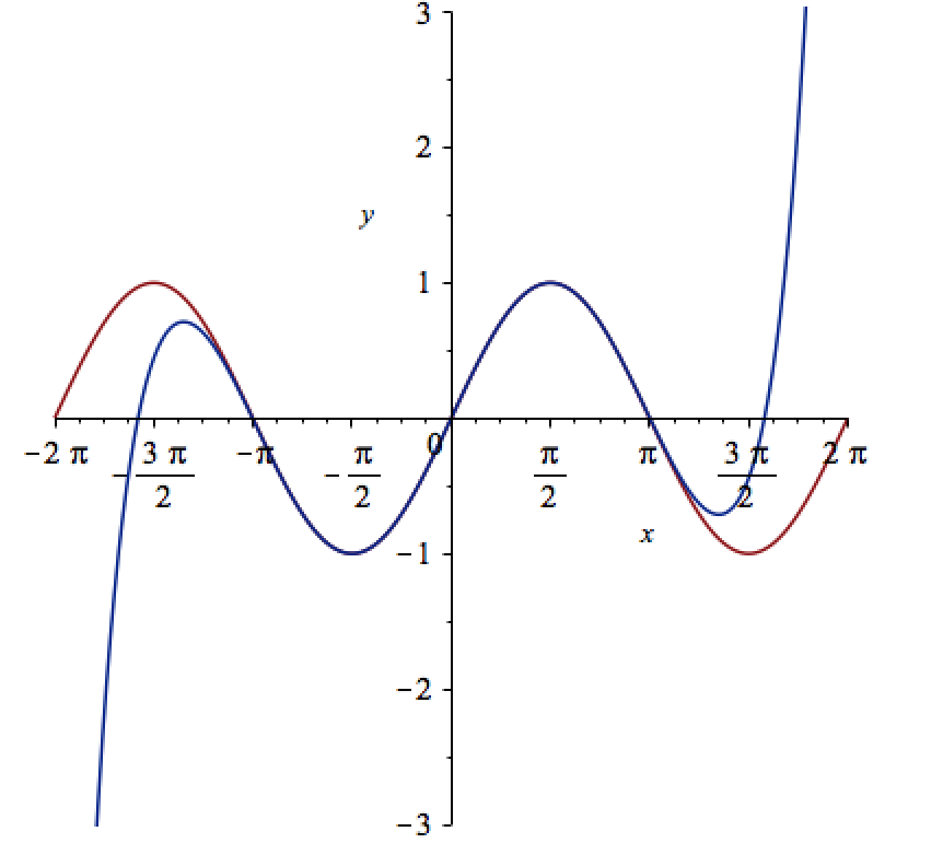
Let’s see how close this is to the sin(x) curve by plotting them both together

plot([sin(x), convert(series(sin(x), x = 0, 10), polynom)], x = -2*Pi .. 2*Pi, y = -3 .. 3);

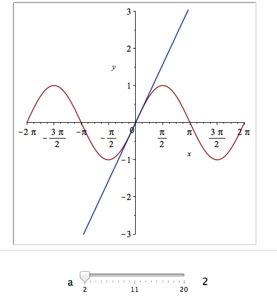
It would be nice if we could see how the approximation varies as we vary the number of terms in the expansion. Change the value 10 to a parameter a, pass the whole thing to the Explore function and we get an interactive widget.

Explore(plot([sin(x), convert(series(sin(x), x = 0, a), polynom)], x = -2*Pi .. 2*Pi, y = -3 .. 3), parameters = [a = 2 .. 20]);

Here’s a screenshot of it:

Adding extra parameters
It would also be nice to vary the point we expand around. Change the value 0 to b and add an extra parameter to Explore to get two sliders instead of one:

Explore(plot([sin(x), convert(series(sin(x), x = b, a), polynom)], x = -2*Pi .. 2*Pi, y = -3 .. 3), parameters = [a = 2 .. 20, b = -2*Pi .. 2*Pi]);

To see what this looks like, open the companion worksheet in Maple.

Adding labels to the sliders
We can change the labels on the sliders as follows

Explore(plot([sin(x), convert(series(sin(x), x = b, a), polynom)], x = -2*Pi .. 2*Pi, y = -3 .. 3), parameters = [[a = 2 .. 20, label = `Number Of Terms`], [b = -2*Pi .. 2*Pi, label = `Expansion location`]]);

To see what this looks like, open the companion worksheet in Maple.

Adding initial values
Finally, let’s set some starting values for each slider

Explore(plot([sin(x), convert(series(sin(x), x = b, a), polynom)], x = -2*Pi .. 2*Pi, y = -3 .. 3), parameters = [[a = 2 .. 20, label = `Number Of Terms`], [b = -2*Pi .. 2*Pi, label = `Expansion location`]], initialvalues = [a = 2, b = 1]);

The resulting interactive widget looks like this:

Not bad for one line of code!

Upload to the Maple Cloud

At The University of Sheffield, we are lucky because all of our staff and students have access to Maple on both university-owned and personally-owned equipment. If your audience isn’t as fortunate, they can access the resulting worksheet on the Maple Cloud.

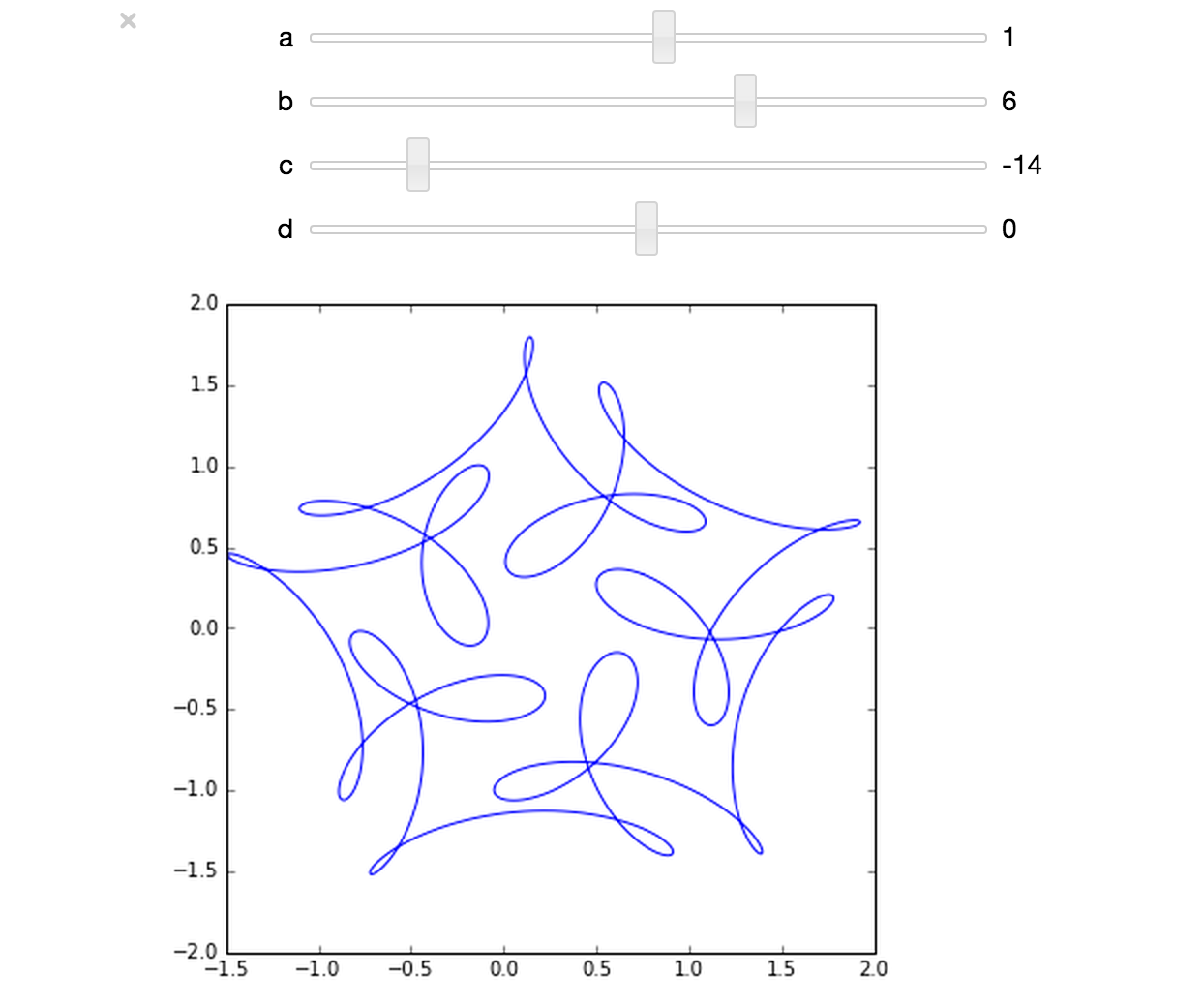
The ever-superb John D. Cook recently found this lovely looking curve in a book he’s currently reading

John posted some Python code that reproduced this curve. I stole borrowed his code, put it in a Jupyter notebook and wrapped it in an interactive widget to allow me to play with the parameters and see what other curves I could come up with. The result looks like this.

If you’d like something where those sliders work, you need to run the notebook I’ve created in Project Jupyter. Here are 2 ways to do that.

• Download the notebook from github
• Method 1: Upload this notebook to Try Jupyter.
• Method 2: Install Anaconda Python on your machine. Launch the notebook and open the file downloaded above.

Once you have the notebook open, click on Cell->Run All and play with the sliders that pop up.

Other posts about these curves:

• Random cyclic curves – Includes code written in Haskell
• A geogebra applet

Update: 2nd July 2015 The code in github has moved on a little since this post was written so I changed the link in the text below to the exact commit that produced the results discussed here.

Imagine that you are a very new MATLAB programmer and you have to create an N x N matrix called A where A(i,j) = i+j
Your first attempt at a solution might look like this

N=2000
% Generate a N-by-N matrix where A(i,j) = i + j;
for ii = 1:N
     for jj = 1:N
         A(ii,jj) = ii + jj;
     end
 end

On my current machine (Macbook Pro bought in early 2015), the above loop takes 2.03 seconds. You might think that this is a long time for something so simple and complain that MATLAB is slow. The person you complain to points out that you should preallocate your array before assigning to it.

N=2000
% Generate a N-by-N matrix where A(i,j) = i + j;
A=zeros(N,N);
for ii = 1:N
     for jj = 1:N
         A(ii,jj) = ii + jj;
     end
 end

This now takes 0.049 seconds on my machine – a speed up of over 41 times! MATLAB suddenly doesn’t seem so slow after all.

Word gets around about your problem, however, and seasoned MATLAB-ers see that nested loop, make a funny face twitch and start muttering ‘vectorise, vectorise, vectorise’. Emails soon pile in with vectorised solutions

% Method 1: MESHGRID.
[X, Y] = meshgrid(1:N, 1:N);
A = X + Y;

This takes 0.025 seconds on my machine — a healthy speed-up on the loop-with-preallocation solution. You have to understand the meshgrid command, however, in order to understand what’s going on here. It’s still clear (to me at least) what its doing but not as clear as the nice,obvious double loop. Call me old fashioned but I like loops…I understand them.

% Method 2: Matrix multiplication.
A = (1:N).' * ones(1, N) + ones(N, 1) * (1:N);

This one is MUCH harder to read but you don’t worry about it too much because at 0.032 seconds it’s slower than meshgrid.

% Method 3: REPMAT.
A = repmat(1:N, N, 1) + repmat((1:N).', 1, N);

This one appears to be interesting! At 0.009 seconds, it’s the fastest so far – by a healthy amount!

% Method 4: CUMSUM.
A = cumsum(ones(N)) + cumsum(ones(N), 2);

Coming in at 0.052 seconds, this cumsum solution is slower than the preallocated loop.

% Method 5: BSXFUN.
A = bsxfun(@plus, 1:N, (1:N).');

Ahhh, bsxfun or ‘The Widow-maker function’ as I sometimes refer to it. Responsible for some of the fastest and most unreadable vectorised MATLAB code I’ve ever written. In this case, it brings execution time down to 0.0045 seconds.

Whenever I see something that can be vectorised with a repmat, I try to figure out if I can rewrite it as a bsxfun. The result is usually horrible to look at so I tend to keep the original loop commented out above it as an explanation! This particular example isn’t too bad but bsxfun can quickly get hairy.

Conclusion

Loops in MATLAB aren’t anywhere near as bad as they used to be thanks to advances in JIT compilation but it can often pay, speed-wise, to switch to vectorisation. The price you often pay for this speed-up is that vectorised code can become very difficult to read.

If you’d like the code I ran to get the timings above, it’s on github (link refers to the exact commit used for this post) . Here’s the output from the run I referred to in this post.

Original loop time is 2.025441
Preallocate and loop is 0.048643
Meshgrid time is 0.025277
Matmul time is 0.032069
Repmat time is 0.009030
Cumsum time is 0.051966
bsxfun time is 0.004527

• MATLAB Version: 2015a
• Early 2015 Macbook Pro with 16Gb RAM
• CPU: 2.8Ghz quad core i7 Haswell

This post is based on a demonstration given by Mathwork’s Ken Deeley during a recent session at The University of Sheffield.

If you really want to learn the differences between Python 2 and Python 3, I suggest you try converting a non-trivial software project. I’m in the middle of doing one now and am learning all kinds of little gotchas over and above the standard stuff that everyone knows such as changes to print, integer division and removal of xrange.

The most recent one I learned about (about 10 minutes ago) amounted to this

#Python 2.7.6 (default, Mar 22 2014, 22:59:56) 
[GCC 4.8.2] on linux2
Type "help", "copyright", "credits" or "license" for more information.
>>> [x for x in range(10)]
[0, 1, 2, 3, 4, 5, 6, 7, 8, 9]
>>> x
9

compared to

Python 3.4.0 (default, Apr 11 2014, 13:05:11) 
[GCC 4.8.2] on linux
Type "help", "copyright", "credits" or "license" for more information.
>>> [x for x in range(10)]
[0, 1, 2, 3, 4, 5, 6, 7, 8, 9]
>>> x
Traceback (most recent call last):
  File "", line 1, in 
NameError: name 'x' is not defined

This is well documented (This StackOverflow Q+A is great!) but I didn’t know about it and, in the code I was looking at, there was a heck of a lot of complication between the list comprehension and when ‘x’ was used. As such, it took me a while to figure out!

Another change that had me scratching my head for a while is the fact that Python 3 ignores the __metaclass__ hook. I didn’t know this little fact but discovered it while debugging failing tests!

Of course, once you know these little gotchas, you’ll probably not be caught out by them again in your next Python 2->Python 3 porting project but they got me wondering…..

What changes from Python 2->Python 3 have really caught you out at some point?

Linear Algebra – Foundations to Frontiers (or LAFF to its friends) is a popular, high quality and free MOOC that, as the title suggests, teaches aspects of linear algebra in a way that takes the student from the very basics through to some cutting edge techniques. I worked through much of it last year and thoroughly enjoyed the approach it took — focusing on programming aspects from the very beginning. The course authors are also among the developers of the FLAME project, a high performance linear algebra library, and one of the interesting aspects of the LAFF course (for me at least) was that it taught linear algebra in a way that also allowed you to understand the approaches used in the algorithms behind FLAME.

Last year, all of the programming assignments in LAFF were done in Python, making use of the IPython notebook. This year, the software stack will be different and will be based on MATLAB. I understand that everyone who signs up to LAFF will be able to get a free MATLAB license from Mathworks for the duration of the course. Understandably, this caused quite a bit of discussion between the LAFF team and software/language geeks like me. In a recent Facebook thread, I asked about the switch and received the reply

‘MATLAB will be free during the course. There are open source equivalents, but Mathworks staff is supporting the use of MATLAB (staff for us). There were some who never got the IPython notebooks to work properly. We are really excited at the opportunity to innovate again and perhaps clear up snags in the programming issues we had. It was complicated to support IPython on all of the operating systems and machines that participants use. MATLAB promises to be easier and will allow us again to concentrate on the Linear Algebra’ – LAFF UTx

I’m sufficiently interested in this change from IPython to MATLAB that I’ll be signing up for the course again this year and I encourage you to do the same — I believe that the programming-centric teaching approach taken by LAFF is extremely well done and your time would be well-spent working through the course.

The course starts on 28th January 2015 so sign up now!

Here’s the trailer for last year’s course.

Given a symmetric matrix such as

What’s the nearest correlation matrix? A 2002 paper by Manchester University’s Nick Higham which answered this question has turned out to be rather popular! At the time of writing, Google tells me that it’s been cited 394 times.

Last year, Nick wrote a blog post about the algorithm he used and included some MATLAB code. He also included links to applications of this algorithm and implementations of various NCM algorithms in languages such as MATLAB, R and SAS as well as details of the superb commercial implementation by The Numerical algorithms group.

I noticed that there was no Python implementation of Nick’s code so I ported it myself.

Here’s an example IPython session using the module

In [1]: from nearest_correlation import nearcorr

In [2]: import numpy as np

In [3]: A = np.array([[2, -1, 0, 0], 
   ...:               [-1, 2, -1, 0],
   ...:               [0, -1, 2, -1], 
   ...:               [0, 0, -1, 2]])

In [4]: X = nearcorr(A)

In [5]: X
Out[5]: 
array([[ 1.        , -0.8084125 ,  0.1915875 ,  0.10677505],
       [-0.8084125 ,  1.        , -0.65623269,  0.1915875 ],
       [ 0.1915875 , -0.65623269,  1.        , -0.8084125 ],
       [ 0.10677505,  0.1915875 , -0.8084125 ,  1.        ]])

This module is in the early stages and there is a lot of work to be done. For example, I’d like to include a lot more examples in the test suite, add support for the commercial routines from NAG and implement other algorithms such as the one by Qi and Sun among other things.

Hopefully, however, it is just good enough to be useful to someone. Help yourself and let me know if there are any problems. Thanks to Vedran Sego for many useful comments and suggestions.

• github repository for the Python NCM module, nearest_correlation
• Nick Higham’s original MATLAB code.
• NAG’s commercial implementation – callable from C, Fortran, MATLAB, Python and more. A superb implementation that is significantly faster and more robust than this one!

I follow a lot of software developers on twitter so I get to see a lot of opinions and comments about git.  Here are a few of my recent favourites

Opinions on git
I find that git is a technology that polarizes people. They either love it or they hate it…often both at the same time.

I didn’t know git would make make programming more addictive. Ups frequency of reward, via miniature accomplishments: commits.

— Alex Holcombe (@ceptional) November 12, 2014

Every time you write, “learn git” and follow this advice with “it’s dead simple!” a kitten cries.

— Anja Boskovic (@damedebugger) November 7, 2014

tries to teach 2 lab groups “git & github” .. actually spends most of the time working on installing/setup. oh Twitter. Just hold me.

— Andrew MacDonald (@polesasunder) November 6, 2014

Git Tutorials
I find that I learn something new every time I read a different tutorial

http://t.co/0OLz7jeghF walkthrough git from internals to (hopefully) better beginners/intermediate usage. Feedback welcomed!

— mrchlblng (@marchelbling) November 12, 2014

[new post] 5 Simple Git Power Tools: http://t.co/bpwRzMJYkx pic.twitter.com/PnAvwW8mcQ

— Jon Reid (@qcoding) November 11, 2014

There’s a new version of the Pro Git Book, and you can read it for free online http://t.co/LaIikATlk1

— Mike Hay (@Hay) November 7, 2014

Git tips and tricks
No matter how long you’ve used git, you can always learn a new trick or two.

duh! Didn’t know about git clean -fdx to clean out gitignored files. I’d been using powershell cmd to del bin/obj & manually del pkg folder

— Julie Lerman (@julielerman) November 6, 2014

alias hadouken="git push origin master -f"

— Chris Oliver (@excid3) November 6, 2014

How to Git Pretty http://t.co/w0CbWYwvvr +@bobthecow pic.twitter.com/AADRNFpuC3

— Elijah Manor (@elijahmanor) November 5, 2014

RLink is Mathematica’s interface to the R language – a feature that has been extremely popular since its debut in Mathematica version 9. It’s a great package but has one or two issues. For example, RLink makes use of a built in version of R which is currently stuck at the rather old version 2.14. Official support for the use of external versions of R and adding third-party libraries varies by operating system and version of Mathematica. Windows support is great — OS X support, not so much.

Expert Mathematica user Szabolcs Horvát has written the definitive guide on how to get RLink up and running with the latest version of R on all three major operating systems, building on earlier work by Leonid Shifrin and members of the Mathematica Stack Exchange community. Thanks to this work, we can now enjoy any version of R we like with Mathematica!

When porting code between MATLAB and Python, it is sometimes useful to produce the exact same set of random numbers for testing purposes.  Both Python and MATLAB currently use the Mersenne Twister generator by default so one assumes this should be easy…and it is…provided you use the generator in Numpy and avoid the seed 0.

Generate some random numbers in MATLAB

Here, we generate the first 5 numbers for 3 different seeds in MATLAB. Our aim is to reproduce these in Python.

>> format long
>> rng(0)
>> rand(1,5)'

ans =

   0.814723686393179
   0.905791937075619
   0.126986816293506
   0.913375856139019
   0.632359246225410

>> rng(1)
>> rand(1,5)'

ans =

   0.417022004702574
   0.720324493442158
   0.000114374817345
   0.302332572631840
   0.146755890817113

>> rng(2)
>> rand(1,5)'

ans =

   0.435994902142004
   0.025926231827891
   0.549662477878709
   0.435322392618277
   0.420367802087489

Python’s default random module

According to the documentation,Python’s random module uses the Mersenne Twister algorithm but the implementation seems to be different from MATLAB’s since the results are different.  Here’s the output from a fresh ipython session:

In [1]: import random

In [2]: random.seed(0)

In [3]: [random.random() for _ in range(5)]
Out[3]: 
[0.8444218515250481,
 0.7579544029403025,
 0.420571580830845,
 0.25891675029296335,
 0.5112747213686085]

In [4]: random.seed(1)

In [5]: [random.random() for _ in range(5)]
Out[5]: 
[0.13436424411240122,
 0.8474337369372327,
 0.763774618976614,
 0.2550690257394217,
 0.49543508709194095]

In [6]: random.seed(2)

In [7]: [random.random() for _ in range(5)]
Out[7]: 
[0.9560342718892494,
 0.9478274870593494,
 0.05655136772680869,
 0.08487199515892163,
 0.8354988781294496]

The Numpy random module

Numpy’s random module, on the other hand, seems to use an identical implementation to MATLAB for seeds other than 0. In the below, notice that for seeds 1 and 2, the results are identical to MATLAB’s. For a seed of zero, they are different.

In [1]: import numpy as np

In [2]: np.set_printoptions(suppress=True)

In [3]: np.set_printoptions(precision=15)

In [4]: np.random.seed(0)

In [5]: np.random.random((5,1))
Out[5]: 
array([[ 0.548813503927325],
       [ 0.715189366372419],
       [ 0.602763376071644],
       [ 0.544883182996897],
       [ 0.423654799338905]])

In [6]: np.random.seed(1)

In [7]: np.random.random((5,1))
Out[7]: 
array([[ 0.417022004702574],
       [ 0.720324493442158],
       [ 0.000114374817345],
       [ 0.30233257263184 ],
       [ 0.146755890817113]])

In [8]: np.random.seed(2)

In [9]: np.random.random((5,1))
Out[9]: 
array([[ 0.435994902142004],
       [ 0.025926231827891],
       [ 0.549662477878709],
       [ 0.435322392618277],
       [ 0.420367802087489]])

Checking a lot more seeds

Although the above interactive experiments look convincing, I wanted to check a few more seeds. All seeds from 0 to 1 million would be a good start so I wrote a MATLAB script that generated 10 random numbers for each seed from 0 to 1 million and saved the results as a .mat file.

A subsequent Python script loads the .mat file and ensures that numpy generates the same set of numbers for each seed. It outputs every seed for which Python and MATLAB differ.

• generate_matlab_randoms.m
• python_randoms.py

On my mac, I opened a bash prompt and ran the two scripts as follows

matlab -nodisplay -nodesktop -r "generate_matlab_randoms"
python python_randoms.py

The output was

MATLAB file contains 1000001 seeds and 10 samples per seed
Random numbers for seed 0 differ between MATLAB and Numpy

System details

• Late 2013 Macbook Air
• MATLAB 2014a
• Python 2.7.7
• Numpy 1.8.1