Walking Randomly

This article is the third part of a series where I look at rewriting a particular piece of MATLAB code using various techniques.  The introduction to the series is here and the introduction to the larger series of GPU articles for MATLAB is here.

Last time I used The Mathwork’s Parallel Computing Toolbox in order to modify a simple correlated asset calculation to run on my laptop’s GPU rather than its CPU.  Performance was not as good as I had hoped and I never managed to get my laptop’s GPU (an NVIDIA GT555M) to beat the CPU using functions from the parallel computing toolbox.  Transferring the code to a much more powerful Tesla GPU card resulted in a four times speed-up compared to the CPU in my laptop.

This time I’ll take a look at AccelerEyes’ Jacket, a third party GPU solution for MATLAB.

Attempt 1 – Make as few modifications as possible

I started off just as I did for the parallel computing toolbox GPU port; by taking the best CPU-only code from part 1 (optimised_corr2.m) and changing a load of data-types from double to gdouble in order to get the calculation to run on my laptop’s GPU using Jacket v1.8.1 and MATLAB 2010b.  I also switched to using the GPU versions of various functions such as grandn instead of randn for example.  Functions such as cumprod needed no  modifications at all since they are nicely overloaded; if the argument to cumprod is of type double then the calculation happens on the CPU whereas if it is gdouble then it happens on the GPU.

Now, one thing that I don’t like about Jacket’s implementation is that many of the functions return single precision numbers by default.  For example, if you do

a=grand(1,10)

then you end up with 10 numbers of type gsingle.  To get double precision numbers you have to do

grandn(1,10,'double')

Now you may be thinking ‘what’s the big deal? – it’s just a bit of syntax so get over it’ and I guess that would be a fair comment.  Supporting single precision also allows users of legacy GPUs to get in on the GPU-accelerated action which is a good thing. The problem as I see it is that almost everything else in MATLAB uses double precision numbers as the default and so it’s easy to get caught out.  I would much rather see functions such as grand return double precision by default with the option to use single precision if required–just like almost every other MATLAB function out there.

The result of my ‘port’ is GPU_jacket_corr1.m

One thing to note in this version, along with all subsequent Jacket versions, is the following command that appears at the very end of the program.

gsync;

This is very important if you want to get meaningful timing results since it ensures that all GPU computations have finished before execution continues. See the Jacket documentation on gysnc and this blog post on timing Jacket code for more details.

The other thing I’ll mention is that, in this version, I do this:

Corr = [1 0.4; 0.4 1];
UpperTriangle=gdouble(chol(Corr));

instead of

Corr = gdouble([1 0.4; 0.4 1]);
UpperTriangle=chol(Corr);

In other words, I do the cholesky decomposition on the CPU and move the results to the GPU rather than doing the calculation on the GPU.  This is mainly because I don’t have access to a Jacket DLA license but it’s probably the best thing to do anyway since such a small decomposition probably won’t happen any faster on the GPU.

So, how does it perform.  I ran it three times with the now usual parameters of 100000 simulations done in blocks of 125 (see the CPU version for how I came to choose 125)

>> tic;GPU_jacket_corr1;toc
Elapsed time is 40.691888 seconds.
>> tic;GPU_jacket_corr1;toc
Elapsed time is 32.096796 seconds.
>> tic;GPU_jacket_corr1;toc
Elapsed time is 32.039982 seconds.

Just like the Parallel Computing Toolbox, the first run is slower because of GPU warmup overheads. Also, just like the PCT, performance stinks! It’s clearly not enough, in this case at least, to blindly throw in a few gdoubles and hope for the best. It is worth noting, however, that this case is nowhere near as bad as the 900+ seconds we saw in the similar parallel computing toolbox version.

Jacket has punished me for being stupid (or optimistic if you want to be polite to me) but not as much as the PCT did.

Attempt 2 – Convert from a script to a function

When working with the Parallel Computing Toolbox I demonstrated that a switch from a script to a function yielded some speed-up.  This wasn’t the case with the Jacket version of the code.  The functional version, GPU_jacket_corr2.m, showed no discernable speed improvement compared to the script.

%Warm up run performed previously
>> tic;GPU_jacket_corr2(100000,125);toc
Elapsed time is 32.230638 seconds.
>> tic;GPU_jacket_corr2(100000,125);toc
Elapsed time is 32.179734 seconds.
>> tic;GPU_jacket_corr2(100000,125);toc
Elapsed time is 32.114864 seconds.

Attempt 3 – One big matrix multiply!

The original version of this calculation performs thousands of very small matrix multiplications and last time we saw that switching to a single, large matrix multiplication brought significant speed improvements on the GPU.  Modifying the code to do this with Jacket is a very similar process to doing it for the PCT so I’ll omit the details and just present the code, GPU_jacket_corr3.m

%Warm up runs performed previously
>> tic;GPU_jacket_corr3(100000,125);toc
Elapsed time is 2.041111 seconds.
>> tic;GPU_jacket_corr3(100000,125);toc
Elapsed time is 2.025450 seconds.
>> tic;GPU_jacket_corr3(100000,125);toc
Elapsed time is 2.032390 seconds.

Now that’s more like it! Finally we have a GPU version that runs faster than the CPU on my laptop. We can do better, however, since the block size of 125 was chosen especially for my CPU. With this Jacket version bigger is better and we get much more speed-up by switching to a block size of 25000 (I run out of memory on the GPU if I try even bigger block sizes).

%Warm up runs performed previously
>> tic;GPU_jacket_corr3(100000,25000);toc
Elapsed time is 0.749945 seconds.
>> tic;GPU_jacket_corr3(100000,25000);toc
Elapsed time is 0.749333 seconds.
>> tic;GPU_jacket_corr3(100000,25000);toc
Elapsed time is 0.749556 seconds.

Now this is exciting! My laptop GPU with Jacket 1.8.1 is faster than a high-end Tesla card using the parallel computing toolbox for this calculation. My excitement was short lived, however, when I looked at the resulting distribution. The random number generator in Jacket 1.8.1 gave a completely different distribution when compared to generators from other sources (I tried two CPU generators from The Mathworks and one from The Numerical Algorithms Group).  The only difference in the code that generated the results below is the random number generator used.

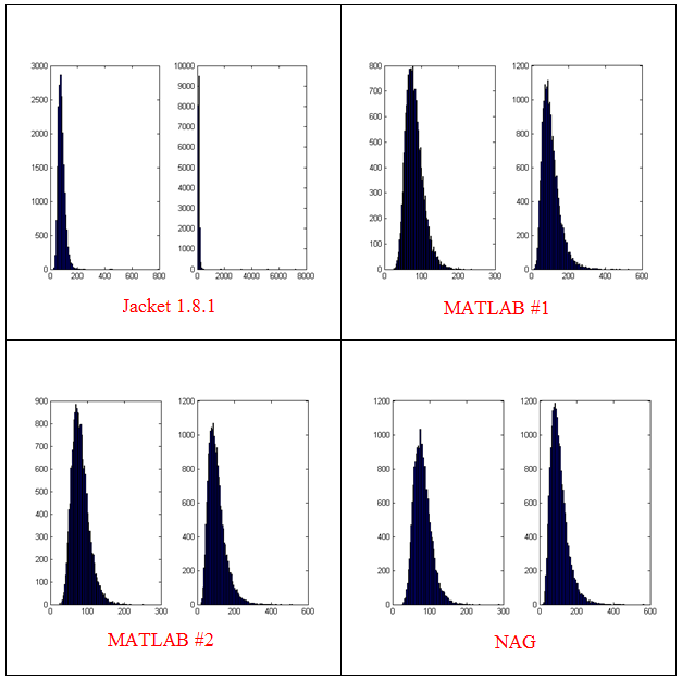
• The results shown in these plots were for only 20,000 simulations rather than the 100,000 I’ve been using elsewhere in this post. I found this bug in the development stage of these posts where I was using a smaller number of simulations.
• Jacket 1.8.1 is using Jackets old grandn function with the ‘double’ option set
• MATLAB #1 is using MATLAB’s randn using the Comb Recursive algorithm on the CPU
• MATLAB #2 is using MATLAB’s randn using the default Mersenne Twister on the CPU
• NAG is using a Wichman-Hill generator

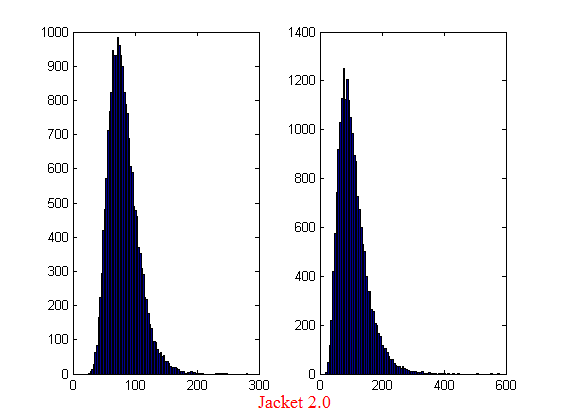
I sent my code to AccelerEye’s customer support who confirmed that this seemed to be a bug in their random number generator (an in-house Mersenne Twister implementation).  Less than a week later they offered me a new preview of Jacket from their Nightly builds where the old RNG had been replaced with the Mersenne Twister implementation produced by NVidia and I’m happy to confirm that not only does this fix the results for my code but it goes even faster!  Superb customer service!

This new RNG is now the default in version 2.0 of Jacket.  Here’s the distribution I get for 20,000 simulations (to stay in line with the plots shown above).

Switching back to 100,000 simulations to stay in line with all of the other benchmarks in this series gives the following times on my laptop’s GPU

%Warm up runs performed previously
>> tic;prices=GPU_jacket_corr3(100000,25000);toc
Elapsed time is 0.696891 seconds.
>> tic;prices=GPU_jacket_corr3(100000,25000);toc
Elapsed time is 0.697596 seconds.
>> tic;prices=GPU_jacket_corr3(100000,25000);toc
Elapsed time is 0.697312 seconds.

This is almost 5 times faster than the 3.42 seconds managed by the best CPU version from part 1. I sent my code to AccelerEyes and asked them to run it on a more powerful GPU, a Tesla C2075, and these are the results they sent back

Elapsed time is 5.246249 seconds. %warm up run
Elapsed time is 0.158165 seconds.
Elapsed time is 0.156529 seconds.
Elapsed time is 0.156522 seconds.
Elapsed time is 0.156501 seconds.

So, the Tesla is 4.45 times faster than my laptop’s GPU for this application and a very useful 21.85 times faster than my laptop’s CPU.

Results Summary

• Best CPU Result on laptop (i7-2630GM)with pure MATLAB code – 3.42 seconds
• Best GPU Result with PCT on laptop (GT555M) – 4.04 seconds
• Best GPU Result with PCT on Tesla M2070 – 0.85 seconds
• Best GPU Result with Jacket on laptop (GT555M) – 0.7 seconds
• Best GPU Result with Jacket on Tesla M2075 – 0.16 seconds

Test System Specification

• Laptop model: Dell XPS L702X
• CPU:Intel Core i7-2630QM @2Ghz software overclockable to 2.9Ghz. 4 physical cores but total 8 virtual cores due to Hyperthreading.
• GPU:GeForce GT 555M with 144 CUDA Cores.  Graphics clock: 590Mhz.  Processor Clock:1180 Mhz. 3072 Mb DDR3 Memeory
• RAM: 8 Gb
• OS: Windows 7 Home Premium 64 bit.
• MATLAB: 2011b

Acknowledgements

Thanks to Yong Woong Lee of the Manchester Business School as well as various employees at AccelerEyes for useful discussions and advice.  Any mistakes that remain are all my own.

Maple has had support for NVidia GPUs since version 14 but I’ve not played with it much until recently.  Essentially I was put off by the fact that Maple’s CUDA package seemed to have support for only one function – Matrix-Matrix Multiplication. However, a recent conversation with a Maple developer changed my mind.

It is true that only MatrixMatrixMultiply has been accelerated but when you flip the CUDA switch in Maple, every function in the LinearAlgebra package that calls MatrixMatrixMultiply also gets accelerated.  This leads to the possibility of a lot of speed-ups for very little work.

So, this morning I thought I would take a closer look using my laptop.  Let’s start by timing how long it takes the CPU to multiply two 4000 by 4000 double precision matrices

with(LinearAlgebra):
CUDA:-Enable(false):
CUDA:-IsEnabled();
a := RandomMatrix(4000, datatype = float[8]):
b := RandomMatrix(4000, datatype = float[8]):
t := time[real]():
c := a.b:
time[real]()-t

The exact time varied a little from run to run but 3.76 seconds is a typical result. I’m only feeling my way at this stage so not doing any proper benchmarking.

To do this calculation on the GPU, all I need to do is change the line

CUDA:-Enable(false):

to

CUDA:-Enable(true):

like so

with(LinearAlgebra):
CUDA:-Enable(true):
CUDA:-IsEnabled();
a := RandomMatrix(4000, datatype = float[8]):
b := RandomMatrix(4000, datatype = float[8]):
t := time[real]():
c := a.b:
time[real]()-t

Typical execution time was 8.37 seconds so the GPU version is more than 2 times slower than the CPU version on my machine.

Trying different matrix sizes

Not wanting to admit defeat after just a single trial, I timed the above code using different matrix sizes.  Here are the results

• 1000 by 1000: CPU=0.07 seconds GPU=0.17 seconds
• 2000 by 2000: CPU=0.53 seconds GPU=1.07 seconds
• 4000 by 4000: CPU=3.76 seconds GPU=8.37 seconds
• 5000 by 5000: CPU=7.44 seconds GPU=19.48 seconds

Switching to single precision

GPUs do much better with single precision numbers so I had a try with those too.  All you need to do is change

datatype = float[8]

to

datatype = float[4]

in the above code. The results are:

• 1000 by 1000: CPU=0.03 seconds GPU=0.07 seconds
• 2000 by 2000: CPU=0.35 seconds GPU=0.66 seconds
• 4000 by 4000: CPU=1.86 seconds GPU=2.37 seconds
• 5000 by 5000: CPU=3.81 seconds GPU=5.2 seconds

So the GPU loses in single precision mode too on my hardware.  If I can’t get a speedup with MatrixMatrixMultiply on my system then there is no point in exploring all of the other LinearAlgebra routines since all of them will be slower when moving to CUDA acceleration.

I guess that in this case, my CPU is too powerful and my GPU is too wimpy to see the acceleration I was hoping for.

Thanks to Maplesoft for providing me with a review copy of Maple 15.

Test System Specification

• Laptop model: Dell XPS L702X
• CPU: Intel Core i7-2630QM @2Ghz software overclockable to 2.9Ghz. 4 physical cores but total 8 virtual cores due to Hyperthreading.
• GPU: GeForce GT 555M with 144 CUDA Cores.  Graphics clock: 590Mhz.  Processor Clock:1180 Mhz. 3072 Mb DDR3 Memeory
• RAM: 8 Gb
• OS: Windows 7 Home Premium 64 bit.
• Maple 15

This article is the second part of a series where I look at rewriting a particular piece of MATLAB code using various techniques.  The introduction to the series is here and the introduction to the larger series of GPU articles for MATLAB on WalkingRandomly is here.

Attempt 1 – Make as few modifications as possible

I took my best CPU-only code from last time (optimised_corr2.m) and changed a load of data-types from double to gpuArray in order to get the calculation to run on my laptop’s GPU using the parallel computing toolbox in MATLAB 2010b.  I also switched to using the GPU versions of various functions such as parallel.gpu.GPUArray.randn instead of randn for example.  Functions such as cumprod needed no  modifications at all since they are nicely overloaded; if the argument to cumprod is of type double then the calculation happens on the CPU whereas if it is gpuArray then it happens on the GPU.

The above work took about a minute to do which isn’t bad for a CUDA ‘porting’ effort!  The result, which I’ve called GPU_PCT_corr1.m is available for you to download and try out.

How about performance?  Let’s do a quick tic and toc using my laptop’s NVIDIA GT 555M GPU.

>> tic;GPU_PCT_corr1;toc
Elapsed time is 950.573743 seconds.

The CPU version of this code took only 3.42 seconds which means that this GPU version is over 277 times slower! Something has gone horribly, horribly wrong!

Attempt 2 – Switch from script to function

In general functions should be faster than scripts in MATLAB because more automatic optimisations are performed on functions.  I didn’t see any difference in the CPU version of this code (see optimised_corr3.m from part 1 for a CPU function version) and so left it as a script (partly so I had an excuse to discuss it here if I am honest).  This GPU-version, however, benefits noticeably from conversion to a function.  To do this, add the following line to the top of GPU_PCT_corr1.m

function [SimulPrices] = GPU_PTC_corr2( n,sub_size)

Next, you need to delete the following two lines

n=100000;                       %Number of simulations
sub_size = 125;

Finally, add the following to the end of our new function

end

That’s pretty much all I did to get GPU_PCT_corr2.m. Let’s see how that performs using the same parameters as our script (100,000 simulations in blocks of 125).  I used script_vs_func.m to run both twice after a quick warm-up iteration and the results were:

Warm up
Elapsed time is 1.195806 seconds.
Main event
script
Elapsed time is 950.399920 seconds.
function
Elapsed time is 938.238956 seconds.
script
Elapsed time is 959.420186 seconds.
function
Elapsed time is 939.716443 seconds.

So, switching to a function has saved us a few seconds but performance is still very bad!

Attempt 3 – One big matrix multiply!

So far all I have done is take a program that works OK on a CPU, and run it exactly as-is on the GPU in the hope that something magical would happen to make it go faster.  Of course, GPUs and CPUs are very different beasts with differing sets of strengths and weaknesses so it is rather naive to think that this might actually work.  What we need to do is to play to the GPUs strengths more and the way to do this is to focus on this piece of code.

for i=1:sub_size
     CorrWiener(:,:,i)=parallel.gpu.GPUArray.randn(T-1,2)*UpperTriangle;
end

Here, we are performing lots of small matrix multiplications and, as mentioned in part 1, we might hope to get better performance by performing just one large matrix multiplication instead. To do this we can change the above code to

%Generate correlated random numbers
%using one big multiplication
randoms = parallel.gpu.GPUArray.randn(sub_size*(T-1),2);
CorrWiener = randoms*UpperTriangle;
CorrWiener = reshape(CorrWiener,(T-1),sub_size,2);
%CorrWiener = permute(CorrWiener,[1 3 2]); %Can't do this on the GPU in 2011b or below

%poor man's permute since GPU permute if not available in 2011b
CorrWiener_final = parallel.gpu.GPUArray.zeros(T-1,2,sub_size);
for s = 1:2
    CorrWiener_final(:, s, :) = CorrWiener(:, :, s);
end

The reshape and permute are necessary to get the matrix in the form needed later on. Sadly, MATLAB 2011b doesn’t support permute on GPUArrays and so I had to use the ‘poor mans permute’ instead.

The result of the above is contained in GPU_PCT_corr3.m so let’s see how that does in a fresh instance of MATLAB.

>> tic;GPU_PCT_corr3(100000,125);toc
Elapsed time is 16.666352 seconds.
>> tic;GPU_PCT_corr3(100000,125);toc
Elapsed time is 8.725997 seconds.
>> tic;GPU_PCT_corr3(100000,125);toc
Elapsed time is 8.778124 seconds.

The first thing to note is that performance is MUCH better so we appear to be on the right track. The next thing to note is that the first evaluation is much slower than all subsequent ones. This is totally expected and is due to various start-up overheads.

Recall that 125 in the above function calls refers to the block size of our monte-carlo simulation. We are doing 100,000 simulations in blocks of 125– a number chosen because I determined empirically that this was the best choice on my CPU. It turns out we are better off using much larger block sizes on the GPU:

>> tic;GPU_PCT_corr3(100000,250);toc
Elapsed time is 6.052939 seconds.
>> tic;GPU_PCT_corr3(100000,500);toc
Elapsed time is 4.916741 seconds.
>> tic;GPU_PCT_corr3(100000,1000);toc
Elapsed time is 4.404133 seconds.
>> tic;GPU_PCT_corr3(100000,2000);toc
Elapsed time is 4.223403 seconds.
>> tic;GPU_PCT_corr3(100000,5000);toc
Elapsed time is 4.069734 seconds.
>> tic;GPU_PCT_corr3(100000,10000);toc
Elapsed time is 4.039446 seconds.
>> tic;GPU_PCT_corr3(100000,20000);toc
Elapsed time is 4.068248 seconds.
>> tic;GPU_PCT_corr3(100000,25000);toc
Elapsed time is 4.099588 seconds.

The above, rather crude, test suggests that block sizes of 10,000 are the best choice on my laptop’s GPU. Sadly, however, it’s STILL slower than the 3.42 seconds I managed on the i7 CPU and represents the best I’ve managed using pure MATLAB code. The profiler tells me that the vast majority of the GPU execution time is spent in the cumprod line and in random number generation (over 40% each).

Trying a better GPU
Of course now that I have code that runs on a GPU I could just throw it at a better GPU and see how that does. I have access to MATLAB 2011b on a Tesla M2070 hooked up to a Linux machine so I ran the code on that. I tried various block sizes and the best time was 0.8489 seconds with the call GPU_PCT_corr3(100000,20000) which is just over 4 times faster than my laptop’s CPU.

Ask the Audience
Can you do better using just the GPU functionality provided in the Parallel Computing Toolbox (so no bespoke CUDA kernels or Jacket just yet)? I’ll be looking at how AccelerEyes’ Jacket myself in the next post.

Results so far

• Best CPU Result on laptop (i7-2630GM)with pure MATLAB code – 3.42 seconds
• Best GPU Result with PCT on laptop (GT555M) – 4.04 seconds
• Best GPU Result with PCT on Tesla M2070 – 0.85 seconds

Test System Specification

• Laptop model: Dell XPS L702X
• CPU: Intel Core i7-2630QM @2Ghz software overclockable to 2.9Ghz. 4 physical cores but total 8 virtual cores due to Hyperthreading.
• GPU: GeForce GT 555M with 144 CUDA Cores.  Graphics clock: 590Mhz.  Processor Clock:1180 Mhz. 3072 Mb DDR3 Memeory
• RAM: 8 Gb
• OS: Windows 7 Home Premium 64 bit.
• MATLAB: 2011b

Acknowledgements

Thanks to Yong Woong Lee of the Manchester Business School as well as various employees at The Mathworks for useful discussions and advice.  Any mistakes that remain are all my own :)

From where I sit it seems that the majority of scientific GPU work is being done with NVIDIA’s proprietary CUDA platform.  All the signs point to the possibility of this changing, however, and I wonder if 2012 will be the year when OpenCL comes of age.  Let’s look at some recent and near future events….

Hardware

• AMD have recently released the AMD Radeon HD 7970, said to be the fastest single- GPU graphics card on the planet.  This new card supports both Microsoft’s DirectCompute along with OpenCL and is much faster than the previous generation of AMD card (see here for compute benchmarks) as well as being faster than NVIDIAs current top of the line GTX 580.
• Intel will release their next generation of CPUs – Ivy Bridge – which will include an increased number of built in GPU cores which should be OpenCL compatible.  Although the current Sandy Bridge processors also contain GPU cores, it is not currently possible to target them with Intel’s OpenCL implementation (version 1.5 is strictly for the CPU cores).  I would be very surprised if Intel didn’t update their OpenCL implementation to be able to target the GPUs in Ivy Bridge this year.
• AMDs latest Fusion processors also contain OpenCL compatible GPU cores directly integrated with the CPU which programmers can exploit using AMD’s Accelerated Parallel Processing (APP) SDK.

The practical upshot of the above is that if a software vendor uses OpenCL to accelerate their product then it could potentially benefit more of their customers than if they used CUDA.  Furthermore, if you want your code to run on the fastest GPU around then OpenCL is the way to go right now.

Software

Having the latest, fastest hardware is pointless if the software you run can’t take advantage of it.  Over the last 12 months I have had the opportunity to speak to developers of various commerical scientific and mathematical software products which support GPU acceleration.  With the exception of Wolfram’s Mathematica, all of them only supported CUDA.  When I asked why they don’t support OpenCL, the response of most of these developers could be paraphrased as ‘The mathematical libraries and vendor support for CUDA are far more developed than those of OpenCL so CUDA support is significantly easier to integerate into our product.‘  Despite this, however, OpenCL support is definitely growing in the world of mathematical and scientific software.

OpenCL in Mathematics software and libraries

• ViennaCL, a GPU-accelerated C++ open-source linear algebra library, was updated to version 1.2.0 on December 31st (just missing the deadline for December’s Month of Math Software).  Roughly speaking, ViennaCL is a mixture of Boost.ublas (high-level interface) and MAGMA (GPU-support), yet based on OpenCL rather than CUDA.
• AccelerEyes released a new major version of their GPU accelerated MATLAB toolbox, Jacket, in late December 2011.  The big news as far as this article is concerned is that it includes support for OpenCL; something that is currently missing from The Mathworks’ Parallel Computing Toolbox.
• Not content with bringing OpenCL support to MATLAB, AccelerEyes also realesed ArrayFire— a free (for the basic version at least) library for C, C++, Fortran, and Python that includes support for both CUDA and OpenCL.
• Although it’s not new news, it’s worth bearing in mind that Mathematica has supported OpenCL for a while now– since the relase of version 8 back in  November 2010.

Finite Element Modelling with Abaqus

• Back in May 2011, Version 6.11 of the finite element modelling package, Abaqus, was released and it included support for NVIDIA cards (see here for NVIDIA’s page on it).  In September, GPU support in Abaqus was broadened to include AMD Hardware with an OpenCL compliant release (see here).

Other projects

• In late December 2011, the first alpha version of FortranCL, an OpenCL interface for Fortran 90, was released.

What do you think?  Will OpenCL start to take the lead in scientific and mathematical software applications this year or will CUDA continue to dominate?  Are there any new OpenCL projects that I’ve missed?

This is part 2 of an ongoing series of articles about MATLAB programming for GPUs using the Parallel Computing Toolbox.  The introduction and index to the series is at https://www.walkingrandomly.com/?p=3730.   All timings are performed on my laptop (hardware detailed at the end of this article) unless otherwise indicated.

Last time

In the previous article we saw that it is very easy to run MATLAB code on suitable GPUs using the parallel computing toolbox.  We also saw that the GPU has its own area of memory that is completely separate from main memory.  So, if you have a program that runs in main memory on the CPU and you want to accelerate part of it using the GPU then you’ll need to explicitly transfer data to the GPU and this takes time.  If your GPU calculation is particularly simple then the transfer times can completely swamp your performance gains and you may as well not bother.

So, the moral of the story is either ‘Keep data transfers between GPU and host down to a minimum‘ or ‘If you are going to transfer a load of data to or from the GPU then make sure you’ve got a ton of work for the GPU to do.‘  Today, I’m going to consider the latter case.

A more complicated elementwise function – CPU version
Last time we looked at a very simple elementwise calculation– taking the sine of a large array of numbers.  This time we are going to increase the complexity ever so slightly.  Consider trig_series.m which is defined as follows

function out = myseries(t)
  out = 2*sin(t)-sin(2*t)+2/3*sin(3*t)-1/2*sin(4*t)+2/5*sin(5*t)-1/3*sin(6*t)+2/7*sin(7*t);
end

Let’s generate 75 million random numbers and see how long it takes to apply this function to all of them.

cpu_x = rand(1,75*1e6)*10*pi;
tic;myseries(cpu_x);toc

I did the above calculation 20 times using a for loop and took the median of the results to get 4.89 seconds¹. Note that this calculation is fully parallelised…all 4 cores of my i7 CPU were working on the problem simultaneously (Many built in MATLAB functions are parallelised these days by the way…No extra toolbox necessary).

GPU version 1 (Or ‘How not to do it’)

One way of performing this calculation on the GPU would be to proceed as follows

cpu_x =rand(1,75*1e6)*10*pi;
tic
%Transfer data to GPU
gpu_x = gpuArray(cpu_x);
%Do calculation using GPU
gpu_y = myseries(gpu_x);
%Transfer results back to main memory
cpu_y = gather(gpu_y)
toc

The mean time of the above calculation on my laptop’s GPU is 3.27 seconds, faster than the CPU version but not by much. If you don’t include data transfer times in the calculation then you end up with 2.74 seconds which isn’t even a factor of 2 speed-up compared to the CPU.

GPU version 2 (arrayfun to the rescue)

We can get better performance out of the GPU simply by changing the line that does the calculation from

gpu_y = myseries(gpu_x);

to a version that uses MATLAB’s arrayfun command.

gpu_y = arrayfun(@myseries,gpu_x);

So, the full version of the code is now

cpu_x =rand(1,75*1e6)*10*pi;
tic
%Transfer data to GPU
gpu_x = gpuArray(cpu_x);
%Do calculation using GPU via arrayfun
gpu_y = arrayfun(@myseries,gpu_x);
%Transfer results back to main memory
cpu_y = gather(gpu_y)
toc

This improves the timings quite a bit. If we don’t include data transfer times then the arrayfun version completes in 1.42 seconds down from 2.74 seconds for the original GPU code. Including data transfer, the arrayfun version complete in 1.94 seconds compared to for the 3.27 seconds for the original.

Using arrayfun for the GPU is definitely the way to go! Giving the GPU every disadvantage I can think of (double precision, including transfer times, comparing against multi-thread CPU code etc) we still get a speed-up of just over 2.5 times on my laptop’s hardware. Pretty useful for hardware that was designed for energy-efficient gaming!

Note: Something that I learned while writing this post is that the first call to arrayfun will be slower than all of the rest.  This is because arrayfun compiles the MATLAB function you pass it down to PTX and this can take a while (seconds).  Subsequent calls will be much faster since arrayfun will use the compiled results.  The compiled PTX functions are not saved between MATLAB sessions.

arrayfun – Good for your memory too!
Using the arrayfun function is not only good for performance, it’s also good for memory management. Imagine if I had 100 million elements to operate on instead of only 75 million. On my 3Gb GPU, the following code fails:

cpu_x = rand(1,100*1e6)*10*pi;
gpu_x = gpuArray(cpu_x);
gpu_y = myseries(gpu_x);
??? Error using ==> GPUArray.mtimes at 27
Out of memory on device. You requested: 762.94Mb, device has 724.21Mb free.

Error in ==> myseries at 3
        out =
        2*sin(t)-sin(2*t)+2/3*sin(3*t)-1/2*sin(4*t)+2/5*sin(5*t)-1/3*sin(6*t)+2/7*sin(7*t);

If we use arrayfun, however, then we are in clover. The following executes without complaint.

cpu_x = rand(1,100*1e6)*10*pi;
gpu_x = gpuArray(cpu_x);
gpu_y = arrayfun(@myseries,gpu_x);

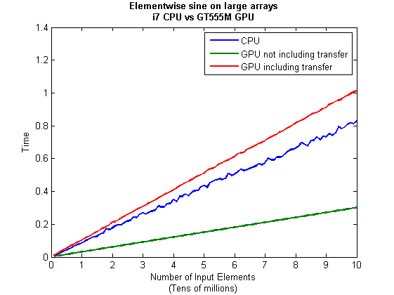
Some Graphs

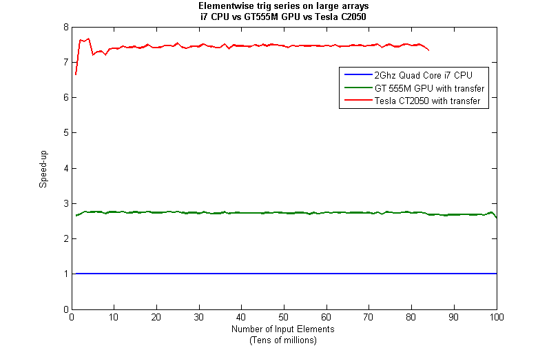
Just like last time, I ran this calculation on a range of input arrays from 1 million to 100 million elements on both my laptop’s GT 555M GPU and a Tesla C2050 I have access to.  Unfortunately, the C2050 is running MATLAB 2010b rather than 2011a so it’s not as fair a test as I’d like.  I could only get up to 84 million elements on the Tesla before it exited due to memory issues.  I’m not sure if this is down to the hardware itself or the fact that it was running an older version of MATLAB.

Next, I looked at the actual speed-up shown by the GPUs compared to my laptop’s i7 CPU.  Again, this includes data transfer times, is in full double precision and the CPU version was multi-threaded (No dodgy ‘GPUs are awesome’ techniques used here).  No matter what array size is used I get almost a factor of 3 speed-up using the laptop GPU and more than a factor of 7 speed-up when using the Tesla.  Not too shabby considering that the programming effort to achieve this speed-up was minimal.

Conclusions

• It is VERY easy to modify simple, element-wise functions to take advantage of the GPU in MATLAB using the Parallel Computing Toolbox.
• arrayfun is the most efficient way of dealing with such functions.
• My laptop’s GPU demonstrated almost a 3 times speed-up compared to its CPU.

Hardware / Software used for the majority of this article

• Laptop model: Dell XPS L702X
• CPU: Intel Core i7-2630QM @2Ghz software overclockable to 2.9Ghz. 4 physical cores but total 8 virtual cores due to Hyperthreading.
• GPU: GeForce GT 555M with 144 CUDA Cores.  Graphics clock: 590Mhz.  Processor Clock:1180 Mhz. 3072 Mb DDR3 Memeory
• RAM: 8 Gb
• OS: Windows 7 Home Premium 64 bit.  I’m not using Linux because of the lack of official support for Optimus.
• MATLAB: 2011a with the parallel computing toolbox

Code and sample timings (Will grow over time)

You need myseries.m and trigseries_test.m and the Parallel Computing Toolbox.  These are the times given by the following function call for various systems (transfer included and using arrayfun).

[cpu,~,~,~,gpu] = trigseries_test(10,50*1e6,'mean')

GPUs

• Tesla C2050, Linux, 2010b – 0.4751 seconds
• NVIDIA GT 555M – 144 CUDA Cores, 3Gb RAM, Windows 7, 2011a – 1.2986 seconds

CPUs

• Intel Core i7-2630QM, Windows 7, 2011a (My laptop’s CPU) – 3.33 seconds
• Intel Core 2 Quad Q9650 @ 3.00GHz, Linux, 2011a – 3.9452 seconds

Footnotes
1 – This is the method used in all subsequent timings and is similar to that used by the File Exchange function, timeit (timeit takes a median, I took a mean). If you prefer to use timeit then the function call would be timeit(@()myseries(cpu_x)). I stick to tic and toc in the article because it makes it clear exactly where timing starts and stops using syntax well known to most MATLABers.

Thanks to various people at The Mathworks for some useful discussions, advice and tutorials while creating this series of articles.

This is part 1 of an ongoing series of articles about MATLAB programming for GPUs using the Parallel Computing Toolbox.  The introduction and index to the series is at https://www.walkingrandomly.com/?p=3730.

Have you ever needed to take the sine of 100 million random numbers?  Me either, but such an operation gives us an excuse to look at the basic concepts of GPU computing with MATLAB and get an idea of the timings we can expect for simple elementwise calculations.

Taking the sine of 100 million numbers on the CPU

Let’s forget about GPUs for a second and look at how this would be done on the CPU using MATLAB.  First, I create 100 million random numbers over a range from 0 to 10*pi and store them in the variable cpu_x;

cpu_x = rand(1,100000000)*10*pi;

Now I take the sine of all 100 million elements of cpu_x using a single command.

cpu_y = sin(cpu_x)

I have to confess that I find the above command very cool. Not only are we looping over a massive array using just a single line of code but MATLAB will also be performing the operation in parallel. So, if you have a multicore machine (and pretty much everyone does these days) then the above command will make good use of many of those cores. Furthermore, this kind of parallelisation is built into the core of MATLAB….no parallel computing toolbox necessary. As an aside, if you’d like to see a list of functions that automatically run in parallel on the CPU then check out my blog post on the issue.

So, how quickly does my 4 core laptop get through this 100 million element array?  We can find out using the MATLAB functions tic and toc. I ran it three times on my laptop and got the following

>> tic;cpu_y = sin(cpu_x);toc
Elapsed time is 0.833626 seconds.
>> tic;cpu_y = sin(cpu_x);toc
Elapsed time is 0.899769 seconds.
>> tic;cpu_y = sin(cpu_x);toc
Elapsed time is 0.916969 seconds.

So the first thing you’ll notice is that the timings vary and I’m not going to go into the reasons why here. What I am going to say is that because of this variation it makes sense to time the calculation a number of times (20 say) and take an average. Let’s do that

sintimes=zeros(1,20);
for i=1:20;tic;cpu_y = sin(cpu_x);sintimes(i)=toc;end
average_time = sum(sintimes)/20

average_time =
    0.8011

So, on average, it takes my quad core laptop just over 0.8 seconds to take the sine of 100 million elements using the CPU.  A couple of points:

• I note that this time is smaller than any of the three test times I did before running the loop and I’m not really sure why.  I’m guessing that it takes my CPU a short while to decide that it’s got a lot of work to do and ramp up to full speed but further insights are welcomed.
• While staring at the CPU monitor I noticed that the above calculation never used more than 50% of the available virtual cores.  It’s using all 4 of my physical CPU cores but perhaps if it took advantage of hyperthreading I’d get even better performance?  Changing OMP_NUM_THREADS to 8 before launching MATLAB did nothing to change this.

Taking the sine of 100 million numbers on the GPU

Just like before, we start off by using the CPU to generate the 100 million random numbers¹

cpu_x = rand(1,100000000)*10*pi;

The first thing you need to know about GPUs is that they have their own memory that is completely separate from main memory. So, the GPU doesn’t know anything about the array created above. Before our GPU can get to work on our data we have to transfer it from main memory to GPU memory and we acheive this using the gpuArray command.

gpu_x = gpuArray(cpu_x); %this moves our data to the GPU

Once the GPU can see all our data we can apply the sine function to it very easily.

gpu_y = sin(gpu_x)

Finally, we transfer the results back to main memory.

cpu_y = gather(gpu_y)

If, like many of the GPU articles you see in the literature, you don’t want to include transfer times between GPU and host then you time the calculation like this:

tic
gpu_y = sin(gpu_x);
toc

Just like the CPU version, I repeated this calculation several times and took an average. The result was 0.3008 seconds giving a speedup of 2.75 times compared to the CPU version.
If, however, you include the time taken to transfer the input data to the GPU and the results back to the CPU then you need to time as follows

tic
gpu_x = gpuArray(cpu_x);
gpu_y = sin(gpu_x);
cpu_y = gather(gpu_y)
toc

On my system this takes 1.0159 seconds on average– longer than it takes to simply do the whole thing on the CPU. So, for this particular calculation, transfer times between host and GPU swamp the benefits gained by all of those CUDA cores.

Benchmark code
I took the ideas above and wrote a simple benchmark program called sine_test.  The way you call it is as follows

[cpu,gpu_notransfer,gpu_withtransfer] = sin_test(numrepeats,num_elements]

For example, if you wanted to run the benchmarks 20 times on a 1 million element array and return the average times then you just do

>> [cpu,gpu_notransfer,gpu_withtransfer] = sine_test(20,1e6)
cpu =
    0.0085
gpu_notransfer =
    0.0022
gpu_withtransfer =
    0.0116

I then ran this on my laptop for array sizes ranging from 1 million to 100 million and used the results to plot the graph below.

But I wanna write a ‘GPUs are awesome’ paper

So far in this little story things are not looking so hot for the GPU  and yet all of the ‘GPUs are awesome’ papers you’ve ever read seem to disagree with me entirely.  What on earth is going on?  Well, lets take the advice given by csgillespie.wordpress.com and turn it on its head.  How do we get awesome speedup figures from the above benchmarks to help us pump out a ‘GPUs are awesome paper’?

0. Don’t consider transfer times between CPU and GPU.

We’ve already seen that this can ruin performance so let’s not do it shall we?  As long as we explicitly say that we are not including transfer times then we are covered.

1. Use a singlethreaded CPU.

Many papers in the literature compare the GPU version with a single-threaded CPU version and yet I’ve been using all 4 cores of my processor.  Silly me…let’s fix that by running MATLAB in single threaded mode by launching it with the command

matlab -singleCompThread

Now when I run the benchmark for 100 million elements I get the following times

>> [cpu,gpu_no,gpu_with] = sine_test(10,1e8)
cpu =
    2.8875
gpu_no =
    0.3016
gpu_with =
    1.0205

Now we’re talking! I can now claim that my GPU version is over 9 times faster than the CPU version.

2. Use an old CPU.

My laptop has got one of those new-fangled sandy-bridge i7 processors…one of the best classes of CPU you can get for a laptop.  If, however, I was doing these tests at work then I guess I’d be using a GPU mounted in my university Desktop machine.  Obviously I would compare the GPU version of my program with the CPU in the Desktop….an Intel Core 2 Quad Q9650.  Heck its running at 3Ghz which is more Ghz than my laptop so to the casual observer (or a phb) it would look like I was using a more beefed up processor in order to make my comparison fairer.

So, I ran the CPU benchmark on that (in singleCompThread mode obviously) and got 4.009 seconds…noticeably slower than my laptop.  Awesome…I am definitely going to use that figure!

I know what you’re thinking…Mike’s being a fool for the sake of it but csgillespie.wordpress.com puts it like this ‘Since a GPU has (usually) been bought specifically for the purpose of the article, the CPU can be a few years older.’ So, some of those ‘GPU are awesome’ articles will be accidentally misleading us in exactly this manner.

3. Work in single precision.

Yeah I know that you like working with double precision arithmetic but that slows GPUs down.  So, let’s switch to single precision.  Just argue in your paper that single precision is OK for this particular calculation and we’ll be set.  To change the benchmarking code all you need to do is change every instance of

rand(1,num_elems)*10*pi;

to

rand(1,num_elems,'single')*10*pi;

Since we are reputable researchers we will, of course, modify both the CPU and GPU versions to work in single precision.  Timings are below

• Desktop at work (single thread, single precision): 3.49 seconds
• Laptop GPU (single precision, not including transfer): 0.122 seconds

OK, so switching to single precision made the CPU version a bit faster but it’s more than doubled GPU performance.  We can now say that the GPU version is over 28 times faster than the CPU version.  Now we have ourselves a bone-fide ‘GPUs are awesome’ paper.

4. Use the best GPU we can find

So far I have been comparing the CPU against the relatively lowly GPU in my laptop.  Obviously, however, if I were to do this for real then I’d get a top of the range Tesla.  It turns out that I know someone who has a Tesla C2050 and so we ran the single precision benchmark on that.  The result was astonishing…0.0295 seconds for 100 million numbers not including transfer times.  The double precision performance for the same calculation on the C2050 was 0.0524 seonds.

5. Write the abstract for our ‘GPUs are awesome’ paper

We took an Nvidia Tesla C2050 GPU and mounted it in a machine containing an Intel Quad Core CPU running at 3Ghz.  We developed a program that performs element-wise trigonometry on arrays of up to 100 million single precision random numbers using both the CPU and the GPU.  The GPU version of our code ran up to 118 times faster than the CPU version.  GPUs are awesome!

Results from different CPUs and GPUs.  Double precision, multi-threaded

I ran the sine_test benchmark on several different systems for 100 million elements.  The CPU was set to be multi-threaded and double precision was used throughout.

sine_test(10,1e8)

GPUs

• Tesla C2050, Linux, 2011a – 0.7487 seconds including transfers,  0.0524 seconds excluding transfers.
• GT 555M – 144 CUDA Cores, 3Gb RAM, Windows 7, 2011a (My laptop’s GPU) -1.0205 seconds including transfers, 0.3016 seconds excluding transfers

CPUs

• Intel Core i7-880 @3.07Ghz, Linux, 2011a – 0.659 seconds
• Intel Core i7-2630QM, Windows 7, 2011a (My laptop’s CPU) – 0.801 seconds
• Intel Core 2 Quad Q9650 @ 3.00GHz, Linux – 0.958 seconds

Conclusions

• MATLAB’s new GPU functions are very easy to use!  No need to learn low-level CUDA programming.
• It’s very easy to massage CPU vs GPU numbers to look impressive.  Read those ‘GPUs are awesome’ papers with care!
• In real life you have to consider data transfer times between GPU and CPU since these can dominate overall wall clock time with simple calculations such as those considered here.  The more work you can do on the GPU, the better.
• My laptop’s GPU is nowhere near as good as I would have liked it to be.  Almost 6 times slower than a Tesla C2050 (excluding data transfer) for elementwise double precision calculations.  Data transfer times seem to about the same though.

Next time

In the next article in the series I’ll look at an element-wise calculation that really is worth doing on the GPU – even using the wimpy GPU in my laptop – and introduce the MATLAB function arrayfun.

Footnote

1 – MATLAB 2011a can’t create random numbers directly on the GPU. I have no doubt that we’ll be able to do this in future versions of MATLAB which will change the nature of this particular calculation somewhat.  Then it will make sense to include the random number generation in the overall benchmark; transfer times to the GPU will be non-existant. In general, however, we’ll still come across plenty of situations where we’ll have a huge array in main memory that needs to be transferred to the GPU for further processing so what we learn here will not be wasted.

Hardware / Software used for the majority of this article

• Laptop model: Dell XPS L702X
• CPU: Intel Core i7-2630QM @2Ghz software overclockable to 2.9Ghz. 4 physical cores but total 8 virtual cores due to Hyperthreading.
• GPU: GeForce GT 555M with 144 CUDA Cores.  Graphics clock: 590Mhz.  Processor Clock:1180 Mhz. 3072 Mb DDR3 Memeory
• RAM: 8 Gb
• OS: Windows 7 Home Premium 64 bit.  I’m not using Linux because of the lack of official support for Optimus.
• MATLAB: 2011a with the parallel computing toolbox

Other GPU articles at Walking Randomly

• GPU Support in Mathematica, Maple, MATLAB and Maple Prime – See the various options available
• Insert new laptop to continue – My first attempt at using the GPU functionality in MATLAB
• NVIDIA lets down Linux laptop users – and how an open source project saves the day

Thanks to various people at The Mathworks for some useful discussions, advice and tutorials while creating this series of articles.

These days it seems that you can’t talk about scientific computing for more than 5 minutes without somone bringing up the topic of Graphics Processing Units (GPUs).  Originally designed to make computer games look pretty, GPUs are massively parallel processors that promise to  revolutionise the way we compute.

A brief glance at the specification of a typical laptop suggests why GPUs are the new hotness in numerical computing.  Take my new one for instance, a Dell XPS L702X, which comes with a Quad-Core Intel i7 Sandybridge processor running at up to 2.9Ghz and an NVidia GT 555M with a whopping 144 CUDA cores.  If you went back in time a few years and told a younger version of me that I’d soon own a 148 core laptop then young Mike would be stunned.  He’d also be wondering ‘What’s the catch?’

Of course the main catch is that all processor cores are not created equally.  Those 144 cores in my GPU are, individually, rather wimpy when compared to the ones in the Intel CPU.  It’s the sheer quantity of them that makes the difference.  The question at the forefront of my mind when I received my shiny new laptop was ‘Just how much of a difference?’

Now I’ve seen lots of articles that compare CPUs with GPUs and the GPUs always win…..by a lot!  Dig down into the meat of these articles,  however, and it turns out that things are not as simple as they seem.  Roughly speaking, the abstract of some them could be summed up as ‘We took  a serial algorithm written by a chimpanzee for an old, outdated CPU and spent 6 months parallelising and fine tuning it for a top of the line  GPU.  Our GPU version is up to 150 times faster!‘

Well it would be wouldn’t it?!  In other news, Lewis Hamilton can drive his F1 supercar around Silverstone faster than my dad can in his clapped out 12 year old van!  These articles are so prevalent that csgillespie.wordpress.com recently published an excellent article that summarised everything you should consider when evaluating them.  What you do is take the claimed speed-up, apply a set of common sense questions and thus determine a realistic speedup.  That factor of 150 can end up more like a factor of 8 once you think about it the right way.

That’s not to say that GPUs aren’t powerful or useful…it’s just that maybe they’ve been hyped up a bit too much!

So anyway, back to my laptop.  It doesn’t have a top of the range GPU custom built for scientific computing, instead it has what Notebookcheck.net refers to as a fast middle class graphics card for laptops.  It’s got all of the required bits though….144 cores and CUDA compute level 2.1 so surely it can whip the built in CPU even if it’s just by a little bit?

I decided to find out with a few randomly chosen tests.  I wasn’t aiming for the kind of rigor that would lead to a peer reviewed journal but I did want to follow some basic rules at least

• I will only choose algorithms that have been optimised and parallelised for both the CPU and the GPU.
• I will release the source code of the tests so that they can be critised and repeated by others.
• I’ll do the whole thing in MATLAB using the new GPU functionality in the parallel computing toolbox.  So, to repeat my calculations all you need to do is copy and paste some code.  Using MATLAB also ensures that I’m using good quality code for both CPU and GPU.

The articles

This is the introduction to a set of articles about GPU computing on MATLAB using the parallel computing toolbox.  Links to the rest of them are below and more will be added in the future.

• Elementwise operations on the GPU #1 – Basic commands using the PCT and how to write a ‘GPUs are awesome’ paper; no matter what results you get!
• Elementwise operations on the GPU #2 – A slightly more involved example showing a useful speed-up compared to the CPU.  An introduction to MATLAB’s arrayfun
• Optimising a correlated asset calculation on MATLAB #1: Vectorisation on the CPU – A detailed look at a port from CPU MATLAB code to GPU MATLAB code.
• Optimising a correlated asset calculation on MATLAB #2: Using the GPU via the PCT – A detailed look at a port from CPU MATLAB code to GPU MATLAB code.
• Optimising a correlated asset calculation on MATLAB #3: Using the GPU via Jacket –  A detailed look at a port from CPU MATLAB code to GPU MATLAB code.

External links of interest to MATLABers with an interest in GPUs

• The Parallel Computing Toolbox (PCT) – The Mathwork’s MATLAB add-on that gives you CUDA GPU support.
• Mike Gile’s MATLAB GPU Blog – from the University of Oxford
• Accelereyes – Developers of ‘Jacket’, an alternative to the parallel computing toolbox.
• A Mandelbrot Set on the GPU – Using the parallel computing toolbox to make pretty pictures…FAST!
• GP-you.org – A free CUDA-based GPU toolbox for MATLAB
• Matlab, CUDA and Me – Stu Blair gives various examples of calling CUDA kernels directly from MATLAB

I recently maxed out my credit card in order to treat myself to a shiny new Dell XPS L720X laptop that comes complete with Intel i7 sandy bridge processor and Nvidia GeForce GT 555M. The NVidia graphics card was one of the biggest selling points for me because I wanted to do some GPU work at home and on the train using both CUDA and OpenCL.  I get asked about these technologies a lot by researchers at The University of Manchester and I wanted to beef up my experience levels.

I wanted this machine to be dual boot Windows 7 and Linux so, before I shelled out my hard-earned cash, I thought I would check that Nvidia’s Linux driver supported the GT 555M. A quick look at their official driver page confirmed that it did so I handed over the credit card. After all, if Nvidia themselves say that it is supported then you’d expect it to be supported right?

Wrong! Here’s my story.

I installed Ubuntu 11.04 from DVD without a hitch and updated all packages to the very latest versions. I then hopped over to NVidia’s website, got the driver (version 275.09.07) and installed it. I’ve gone through this process dozens of times on Desktop machines at work and wasn’t expecting any problems but boy did I get problems. After installing NVidia’s driver, the Dell simply would not boot into Linux. Not only that but it never seemed to fail in exactly the same place twice…the boot process would start just fine and then it would crash…seemingly at random.  So, off to the forums I went where I quickly discovered that my system was not as supported as I originally thought.

You see, my laptop has two graphics systems on it: A relatively low-powered Intel one and the NVidia one. It also comes with some cool sounding technology called Optimus that helps save battery power on systems like mine. Rather than explain the details of Optimus, I’m just going to refer you to both Nvidia’s web page about it along with the Wikipedia page.

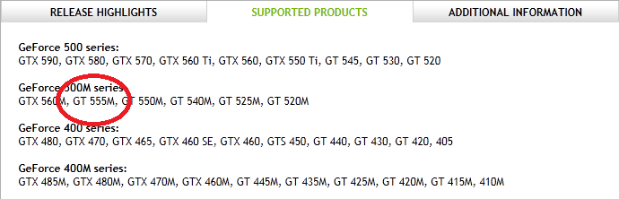
Here’s the kicker…Nvidia’s Linux driver does not support optimus, even though Optimus is Nvidia’s own technology. They even say that they don’t support it in the Additional Information tab. Furthermore, they have no plans to support it.  Sadly, I didn’t even realise that my new laptop was an Optimus laptop until I tried to get the Nvidia drivers on it.

If only I had thought to myself ‘Well, Nvidia may say that they support the 555M but do they really mean it?’ If I mis-trusted the information given on the supported products page then perhaps then I would have read the further information tab and trawled the forums. I chose to trust Nvidia and assume that when a product was listed under ‘supported products’ then I didn’t need to worry. Well you live and learn I guess.

Project Bumblebee

One of the fantastic things about the Linux community is that even if you are let down by your hardware vendor then someone, somewhere may well come to your rescue. For Nvidia Optimus, that someone is Martin Juhl. Martin’s project, Bumblebee, brings Optimus support to Linux which is useful since it seems that Nvidia can’t be bothered!

Installation for Ubuntu users is easy.  All you need to do is open up a terminal, type the following and follow the instructions to download and install both the Nvidia drivers along with bumblebee.

sudo apt-add-repository ppa:mj-casalogic/bumblebee
sudo apt-get update && sudo apt-get install bumblebee

To run an application, glxgears for example, you just type the following at the command line

optirun glxgears

Sadly for me this didn’t work.  All I got was the following

 * Starting Bumblebee X server bumblebee
_PS0 Enabling nVidia Card Succeded. [ OK ]

 * Stopping Bumblebee X server bumblebee
_DSM Disabling nVidia Card Succeded.
_PS3 Disabling nVidia Card Succeded.

Nothing else happened. I’d report it as a bug-report but it seems that someone with a very similar configuration to me has already done so and work is being done on it as we speak.  Plenty of other people have reported success with bumblebee though and I am confident that I will be up and running soon.  As soon as I am up and running I’ll owe the developer of bumblebee a beer!

Update 11th July: The bumblebee bug mentioned above has been fixed.  I can now run apps via optirun.  Not done much more than run glxgears though so far.

Updated January 4th 2011

It is becoming increasingly common for programmers to make use of GPUs (Graphical Processing Units) to speed up their programs substantially.  There are three major low-level programming libraries that allow you to do this in languages such as C; namely CUDA, OpenCL and Microsoft DirectCompute.  Of these three, CUDA is the most developed but it only works on Nvidia graphics cards.

I am often asked if the major commercial math packages support GPU computing and I find myself writing the same summary email over and over again.  So, here is a very brief breakdown of what is currently on offer.  I plan to expand the information contained in this page over time so if you have any information about GPU computing in these packages then let me know.

MATLAB

Core MATLAB contains no support for GPU computing but several organizations (including The Mathworks themselves) have produced add-on toolboxes that add such support:

• Jacket – This is a product from a company called AccelerEyes and is possibly the most advanced and well developed GPU solution for MATLAB currently available.  As of version 2.0 it supports both OpenCL and CUDA frameworks.
• The Mathworks’ Parallel Computing Toolbox (PCT) – If you want to do your MATLAB GPU computing the officially supported way then this is the product you need.  As a bonus, it also allows you to make better use of the multicore processor that almost certainly resides in your machine.  Like many of the offerings on this page, only the CUDA framework is supported so you are out of luck if you don’t have an NVidia graphics card.  Even if you do have an NVidia graphics card then you still might be out of luck since the PCT only supports cards that have compute level 1.3 or above (i.e. double precision only).
• CULA is a set of GPU-accelerated linear algebra libraries utilizing the NVIDIA CUDA parallel computing architecture and it has a MATLAB interface.
• GPUmat – This product is completely free but is less developed than the commercial offerings above.  Again. it is CUDA only
• OpenCL toolbox – The only OpenCL solution for MATLAB I could find.  It is free but development seems to have stalled.

Mathematica

Mathematica 8 has support for both CUDA and OpenCL built in so no need for any add-ons.  Furthermore, it supports both single and double precision GPUs so you can experiment with GPU computing on older, cheaper cards.

Maple

Maple has had some CUDA-only GPU support since version 14.  On the face of it, the CUDA package only appears to contain one accelerated function–Matrix-Matrix multiplication– but when you load this function it accelerates many functions that use matrix-matrix multiply internally.  I’ve never found a definitive list of such functions though.

Mathcad

Mathcad 15 and Mathcad Prime have no support for GPU enhanced computing.