
Archive for the ‘math software’ Category
While working on someone’s MATLAB code today there came a point when it was necessary to generate a vector of powers. For example, [a a^2 a^3….a^10000] where a=0.999
a=0.9999;
y=a.^(1:10000);
This isn’t the only way one could form such a vector and I was curious whether or not an alternative method might be faster. On my current machine we have:
>> tic;y=a.^(1:10000);toc
Elapsed time is 0.001526 seconds.
>> tic;y=a.^(1:10000);toc
Elapsed time is 0.001529 seconds.
>> tic;y=a.^(1:10000);toc
Elapsed time is 0.001716 seconds.
Let’s look at the last result in the vector y
>> y(end)
ans =
   0.367861046432970
So, 0.0015-ish seconds to beat.
>> tic;y1=cumprod(ones(1,10000)*a);toc
Elapsed time is 0.000075 seconds.
>> tic;y1=cumprod(ones(1,10000)*a);toc
Elapsed time is 0.000075 seconds.
>> tic;y1=cumprod(ones(1,10000)*a);toc
Elapsed time is 0.000075 seconds.
soundly beaten! More than a factor of 20 in fact. Let’s check out that last result
>> y1(end)
ans =
   0.367861046432969
Only a difference in the 15th decimal place–I’m happy with that. What I’m wondering now, however, is will my faster method ever cause me grief?
This is only an academic exercise since this is not exactly a hot spot in the code!
In common with many higher educational establishments, the University I work for has site licenses for a wide variety of scientific software applications such as Labview, MATLAB, Mathematica, NAG, Maple and Mathcad— a great boon to students and researcher who study and work there. The computational education of a typical STEM undergraduate will include exposure to at least some of these systems along with traditional programming languages such as Java, C or Fortran and maybe even a little Excel when times are particularly bad!
Some argue that such exposure to multiple computational systems is a good thing while others argue that it leads to confusion and a ‘jack of all trades and master of none situation.’ Those who take the latter viewpoint tend to want to standardize on one system or other depending on personal preferences and expertise.
MATLAB, Python, Fortran and Mathematica are a few systems I’ve seen put forward over the years with the idea being that students will learn the basics of one system in their first few weeks and then the entire subject curriculum will be interwoven with these computational skills. In this way, students can use their computational skills as an aid to deeper subject understanding without getting bogged down with the technical details of several different computational systems. As you might expect, software vendors are extremely keen on this idea and will happily parachute in a few experts to help universities with curriculum development for free since this will possibly lead to their system being adopted.
Maybe we’ll end up with electrical engineers who’ve only ever seen Labview, mathematicians who’ve only ever used Maple, mechanical engineers who’ve only ever used MATLAB and economists who can only use Excel. While the computational framework(s) used to teach these subjects are less important than the teaching of the subject itself, I firmly believe that part of a well-rounded, numerate education should include exposure to several computational systems and such software mono-cultures should be avoided at all costs.
Part of the reason for writing this post is to ask what you think so comments are very welcome.
A colleague recently sent me this issue. Consider the following integral

Attempting to evaluate this with Mathematica 9 gives 0:
 f[a_, b_] := Exp[I*(a*x^3 + b*x^2)];
Integrate[f[a, b], {x, -Infinity, Infinity},
 Assumptions -> {a > 0, b \[Element] Reals}]

Out[2]= 0
So, for all valid values of a and b, Mathematica tells us that the resulting integral will be 0.
However, Let’s set a=1/3 and b=0 in the function f and ask Mathematica to evaluate that integral
In[3]:= Integrate[f[1/3, 0], {x, -Infinity, Infinity}]

Out[3]= (2*Pi)/(3^(2/3)*Gamma[2/3])
This is definitely not zero as we can see by numerically evaluating the result:
In[5]:=
(2*Pi)/(3^(2/3)*Gamma[2/3])//N

Out[5]= 2.23071
Similarly if we put a=1/3 and b=1 we get another non-zero result
In[7]:= Integrate[f[1/3, 1], {x, -Infinity, Infinity}] // InputForm

Out[7]=2*E^((2*I)/3)*Pi*AiryAi[-1]

In[8]:=
2*E^((2*I)/3)*Pi*AiryAi[-1]//N

Out[8]= 2.64453 + 2.08083 I
We are faced with a situation where Mathematica is disagreeing with itself. On one hand, it says that the integral is 0 for all a and b but on the other it gives non-zero results for certain combinations of a and b. Which result do we trust?
One way to proceed would be to use the NIntegrate[] function for the two cases where a and b are explicitly defined. NIntegrate[] uses completely different algorithms from Integrate. In particular it uses numerical rather than symbolic methods (apart from some symbolic pre-processing).
NIntegrate[f[1/3, 0], {x, -Infinity, Infinity}]
gives 2.23071 + 0. I and
NIntegrate[f[1/3, 1], {x, -Infinity, Infinity}]
gives 2.64453 + 2.08083 I
What we’ve shown here is that evaluating these integrals using numerical methods gives the same result as evaluating using symbolic methods and numericalizing the result. This gives me some confidence that its the general, symbolic evaluation that’s incorrect and hence I can file a bug report with Wolfram Research.
Maple 17.01 on the general problem
Since my University has just got a site license for Maple, I wondered what Maple 17.01 would make of the general integral. Using Maple’s 1D input/output we get:
> myint := int(exp(I*(a*x^3+b*x^2)), x = -infinity .. infinity);

myint := (1/12)*3^(1/2)*2^(1/3)*((4/3)*Pi^(5/2)*(((4/27)*I)*b^3/a^2)^(1/3)*exp(((2/27)*I)*b^3/a^2)
*BesselI(-1/3, ((2/27)*I)*b^3/a^2)+((2/3)*I)*Pi^(3/2)*3^(1/2)*b*2^(2/3)
*hypergeom([1/2, 1], [2/3, 4/3],((4/27)*I)*b^3/a^2)/(-I*a)^(2/3)-(8/27)*2^(1/3)*Pi^(5/2)*b^2*
exp(((2/27)*I)*b^3/a^2)*BesselI(1/3, ((2/27)*I)*b^3/a^2)/((-I*a)^(4/3)*(((4/27)*I)*b^3/a^2)^(1/3)))
/(Pi^(3/2)*(-I*a)^(1/3))+(1/12)*3^(1/2)*2^(1/3)*((4/3)*Pi^(5/2)*(((4/27)*I)*b^3/a^2)
^(1/3)*exp(((2/27)*I)*b^3/a^2)*BesselI(-1/3, ((2/27)*I)*b^3/a^2)+((2/3)*I)*Pi^(3/2)*3^(1/2)*b*2^(2/3)
*hypergeom([1/2, 1], [2/3, 4/3], ((4/27)*I)*b^3/a^2)/(I*a)^(2/3)-(8/27)*2^(1/3)*Pi^(5/2)*b^2*
exp(((2/27)*I)*b^3/a^2)*BesselI(1/3, ((2/27)*I)*b^3/a^2)/((I*a)^(4/3)*(((4/27)*I)*b^3/a^2)^(1/3)))
/(Pi^(3/2)*(I*a)^(1/3))
That looks scary! To try to determine if it’s possibly a correct general result, let’s turn this expression into a function and evaluate it for values of a and b we already know the answer to.
>f := unapply(%, a, b):
>result1:=simplify(f(1/3,1));

result1 := (2/27)*3^(1/2)*Pi*exp((2/3)*I)*((-(1/3)*I)^(1/3)*3^(2/3)*(-1)^(1/6)*BesselI(-1/3, (2/3)*I)
+3*(-(1/3)*I)^(2/3)*BesselI(-1/3, (2/3)*I)+3*(-(1/3)*I)^(2/3)*BesselI(1/3, (2/3)*I)-BesselI(1/3, (2/3)*I)
*3^(1/3)*(-1)^(1/3))/(-(1/3)*I)^(2/3)

evalf(result1);
2.644532853+2.080831872*I
Recall that Mathematica returned 2*E^((2*I)/3)*Pi*AiryAi[-1]=2.64453 + 2.08083 I for this case. The numerical results agree to the default precision reported by both packages so I am reasonably confident that Maple’s general solution is correct.
Not so simple simplification?
I am also confident that Maple’s expression involving Bessel functions is equivalent to Mathematica’s expression involving the AiryAi function. I haven’t figured out, however, how to get Maple to automatically reduce the Bessel functions down to AiryAi. I can attempt to go the other way though. In Maple:
>convert(2*exp((2*I)/3)*Pi*AiryAi(-1),Bessel);

(2/3)*exp((2/3)*I)*Pi*(-1)^(1/6)*(-BesselI(1/3, (2/3)*I)*(-1)^(2/3)+BesselI(-1/3, (2/3)*I))
This is more compact than the Bessel function result I get from Maple’s simplify so I guess that Maple’s simplify function could have done a little better here.
Not so general general solution?
Maple’s solution of the general problem should be good for all a and b right? Let’s try it with a=1/3, b=0
f(1/3,0);
Error, (in BesselI) numeric exception: division by zero
Uh-Oh! So it’s not valid for b=0 then! We know from Mathematica, however, that the solution for this particular case is (2*Pi)/(3^(2/3)*Gamma[2/3])=2.23071. Indeed, if we solve this integral directly in Maple, it agrees with Mathematica
>myint := int(exp(I*(1/3*x^3+0*x^2)), x = -infinity .. infinity);

myint := (2/9)*3^(5/6)*(-1)^(1/6)*Pi/GAMMA(2/3)-(2/9)*3^(5/6)*(-1)^(5/6)*Pi/GAMMA(2/3)

>simplify(myint);
(2/3)*3^(1/3)*Pi/GAMMA(2/3)

>evalf(myint);
2.230707052+0.*I
Going to back to the general result that Maple returned. Although we can’t calculate it directly, We can use limits to see what its value would be at a=1/3, b=0
>simplify(limit(f(1/3, x), x = 0));

(2/9)*Pi*3^(2/3)/((-(1/3)*I)^(1/3)*GAMMA(2/3)*((1/3)*I)^(1/3))

>evalf(%)

evalf(%);
2.230707053+0.1348486379e-9*I
The symbolic expression looks different and we’ve picked up an imaginary part that’s possibly numerical noise. Let’s use more numerical precision to see if we can make the imaginary part go away. 100 digits should do it
>evalf[100](%%);

2.230707051824495741427486519543450239771293806030489125938415383976032081571780278667202004477941904
-0.855678513686459467847075286617333072231119978694352241387724335424279116026690601018858453303153701e-100*I
Well, more precision has made the imaginary part smaller but it’s still there. No matter how much precision I use, it’s always there…getting smaller and smaller as I ramp up the level of precision.
What’s going on?
All I’m doing here is playing around with the same problem in two packages. Does anyone have any further insights into some of the issues raised?
I recently picked up a few control theory books from the University library to support a project I am involved with right now and was interested in the seemingly total dominance of MATLAB in this subject area. Since I’m not an expert in control systems, I’m not sure if this is because MATLAB is genuinely the best tool for the job or if it’s simply because it’s been around for a very long time and so has become entrenched. Comments from anyone who works in relevant fields would be most welcome.
On its own, MATLAB is insufficient to teach introductory control systems courses — you also need the control systems toolbox as a bare minimum but most books and courses also seem to require Simulink and the symbolic math toolbox. All of these are included in the student edition of MATLAB which is very reasonably priced.
If you are not a registered student, however, and don’t work for someone who can provide you with MATLAB it’s going to be very expensive! As far as I can tell, your only option would be to purchase commercial licenses which are very expensive (as in thousands of dollars/pounds for MATLAB and a few toolboxes).
What else is out there?
I have a strong interest in mathematical software and so I know that there are several products that have support for control theory. Here are some that I know of and have access to myself
- Mathematica – Its symbolic math support far exceeds that of MATLAB and it is on an equal footing numerically but its control systems support is much more recent and I don’t know of a textbook that utilizes it. One benefit of Mathematica is that it doesn’t separate functionality out into toolboxes – everything is just built in. Another benefit to tinkerers is the home edition which gives you the full product at a much lower price than commercial licenses.
- Maple – This also has very strong symbolic and numeric math support. It also comes with some Control Systems support built in. Like Mathematica, it has a home edition for non-commercial tinkering and learning.
- Labview – A graphical programming language that I’m only just starting to get used to. It has lots of users and advocates in my employers electrical and mechanical engineering departments. There is no support for symbolic computing as far as I know.
- Python – Python is a superb general purpose scripting language that’s also completely free. Numerics are taken care of by Numpy, symbolics by Sympy and there is a control theory module, the development of which is coordinated by Richard Murray of Caltech (The same Richard Murray that co-wrote the book Feedback Systems: An Introduction for Scientists and Engineers).
- Octave – Octave is a free implementation of the MATLAB .m language. It also has a free control package.
- Scilab – Scilab is a free numerical environment that also has a free control package.
I haven’t mentioned Simulink alternatives in this post since I’ve discussed them before.
Questions
Some questions that arise are
- Are there any other alternatives to those listed above?
- Do these alternatives have sufficient functionality to support undergraduate courses in control systems and control theory?
- What would be the best language to use if you were teaching control systems as a Massively Open Online Course (MOOC)?
- Does it matter to employers which computational language you learned your control systems in as an undergraduate?
I find that the final point is very divisive among people I discuss it with. On the one hand you have those who say ‘It’s the concepts that matter, the language you choose to implement them in is much less important’ and on the other hand you have those who say ‘It’s gotta be MATLAB, my father used MATLAB and his grandfather before him. Industry uses MATLAB, I only know MATLAB, we must teach MATLAB.’
As I type this, the sun is shining (finally!) and the skies are blue. You’d think that it would be difficult to concentrate on writing this Month’s mathematical software round-up but it has been such an interesting month that it turned out to be a breeze. Thanks to everyone who submitted news items for this month’s review, your feedback and generosity is greatly appreciated–I would have given up long ago without it.
If you have any news items for next month’s issue, please let me know via the usual channels. Click here for the Month of Math Software Archives.
Things that are a bit like MATLAB
- Rene grothmann’s free Euler Math Toolbox is so frequently updated that it almost always features in these software round-ups. The project is now at version 22.1 and it now others support for Python among other things. See what’s new by clicking on http://euler.rene-grothmann.de/Programs/Changes.html
- A new minor release of Scilab, the free MATLAB-like system from Scilab Enterprises, is now available. To see what’s new in version 5.4.1, head over to https://www.scilab.org/community/news/20130402
Things written for MATLAB
- GAGA: GPU Accelerated Greedy Algorithms for Compressed Sensing is “a software package for solving large compressed sensing problems with millions of unknowns in fractions of a second by exploiting the power of graphics processing units”. It saw its first ever release in April.
- Version 3.4.3.3481 of the Multiprecision Computing Toolbox for MATLAB was released in April bringing several enhancements including the addition of the incomplete gamma function, improvement to the accuracy of eigensolvers and speed up of determinant computations.
Spreadsheets
- One of the most famous spreadsheet errors of all time was unearthed this month. I’ll leave the explaining to the BBC and New Scientist.
- Gnumeric is the free spreadsheet program from the GNOME Office project and April saw it updated to version 1.12.2 Updates include a set of new computational functions, fixes to various file import tools and a new font selector.
Graphs and Plotting
- GNUPlot is a free, open source plotting package that’s been around for over 25 years. It has been ported to almost every computer system known to man including Ye Olde Windows Mobile, Android and Raspberry Pi along with all of the platforms you’d usually expect. April 2013 saw version 4.6.3 and the list of changes is at http://www.gnuplot.info/announce_4.6.3.txt
- DISLIN is a plotting library for C, Fortran 77 and Fortran 90/95 and is also callable from several other languages including Perl,Python and Java. Developed by the Max Plank Institute for Solar System Research, DISLIN has just hit version number 10.3.2. Take a look at the new goodness here.
Numerical libraries
- The 2013 version of the HSL Software Library is now available. The full list of changes, additions and improvements is available at http://www.hsl.rl.ac.uk/changes.html
Python
It’s been a big month for mathematical and scientific software in Python with several releases of note.
- After 7 months of work, The SciPy team have unveiled version 0.12.0. The full list of updates is at http://sourceforge.net/projects/scipy/files/scipy/0.12.0/ but standout features for me are a Basin Hopping Global Optimisation routine (never heard of that algorithm but sounds interesting), the ability to inspect the contents of MATLAB .mat files without actually reading them to memory and documented BLAS and LAPACK low-level interfaces.
- According to its website, numexpr “evaluates multiple-operator array expressions many times faster than NumPy can.” In other words, numexpr is one way to get Python code going faster. Something that I didn’t realise until I wrote this entry is that it supports the high performance Intel Vector Math Library (VML). April saw a release to version 1.4.2 with the new stuff listed at https://code.google.com/p/numexpr/wiki/ReleaseNotes
- Pweave is a scientific report generator and a literate programming tool for Python, inspired by Sweave for R. Version 0.21.2 of Pweave was released earlier this month — take a look at the release notes for details of what’s new. Thanks to @mpastell for the news.
- The IPython (Interactive computing in Python) team have released a bugfix update. The details of version 0.13.2 are in the release notes.
- Version 1.0 of the PyASTRAToolbox was released on 23rd April. “The PyASTRAToolbox is a Python interface to the ASTRA Toolbox, a tomography toolbox based on high-performance GPU primitives for 2D and 3D tomography.”
Misc
- Derek of Coding-guidelines.com has released version 0.5 of his Numbers tool which looks at the numeric literals contained in the source code of any program you pass to it. The numbers program extracts these literals, compares them against a database of ‘interesting’ values and prints out any matches; it can also print out values that don’t match. The matching is fuzzy, the intent being to find mistakes. To see why this might be interesting and useful, take a look at this blog post where Derek discovers that both Maxima and R use a wide variety of different literal values for pi.
- Version 2.19-5 of Magma, the regularly updated, commercial computer algebra system with a focus on algebra, number theory, algebraic geometry and algebraic combinatorics has been released.
- Version 6.1 of MapleSim has been released. MapleSim is a physical modeling and simulation tool.
From the blogs
- Recognizing Numbers – This is very cool! Use Python’s sympy to discover formulas for numbers. For example, to discover that an approximation to pi is exp(141/895 + sqrt(780631)/895)
- Distributed Numerical Optimization in Julia – “This post walks through the parallel computing functionality of Julia to implement an asynchronous parallel version of the classical cutting-plane algorithm for convex (nonsmooth) optimization, demonstrating the complete workflow including running on both Amazon EC2 and a large multicore server”
- High Performance Polynomials in Maple 17 – 75 times faster than Factor in Mathematica 9 apparently according to this blog post.
- ArrayFire Examples (Part 4 of 8) – Image Processing – If you have a GPU and are interested in Image Processing, this is well worth your time.
- History of the modern graphics processor – From video games to high performance research computing.
- Data Science of the Facebook World – Mathematica + Facebook = interesting stuff.
- Using Symbolic Math Toolbox to Compute Area Moment of Intertia
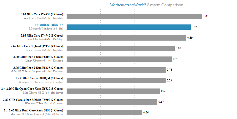
A friend of mine recently got hold of a Microsoft Surface Pro tablet and he let me have a play on it for a couple of hours. So, I installed Mathematica 9 and ran the benchmark. A screenshot of the result is below with the Surface’s result in blue. Not bad for a tablet!
Touch controlled Manipulates were a lot of fun too. If only I could run such things on my iPad as appeared to be promised in http://blog.wolfram.com/2012/02/17/a-preview-of-cdf-on-ipad/
My only other comment is that the Touch Cover is truly awful, reminding me of ye-olde ZX81, but I’ve been told that the Type Cover is much better
Welcome to the latest Month of Math Software here at WalkingRandomly. If you have any mathematical software news or blogposts that you’d like to share with a larger audience, feel free to contact me. Thanks to everyone who contributed news items this month, I couldn’t do it without you.
The NAG Library for Java
- The Numerical Algorithms Group (NAG) have been producing numerical libraries for over 40 years and now they have one for Java.
MATLAB-a-likes
- Version 3.6.4 of Octave, the free, open-source MATLAB clone has been released. This version contains some minor bug fixes. To see everything that’s new since version 3.6, take a look at the NEWS file. If you like MATLAB syntax but don’t like the price, Octave may well be for you.
- The frequently updated Euler Math Toolbox is now at version 20.98 with a full list of changes in the log. Scanning through the recent changes log, I came across the very nice iteratefunction which works as follows
>iterate("cos(x)",1,100,till="abs(cos(x)-x)<0.001")

[ 1  0.540302305868  0.857553215846  0.654289790498  0.793480358743
0.701368773623  0.763959682901  0.722102425027  0.750417761764
0.731404042423  0.744237354901  0.735604740436  0.74142508661
0.737506890513  0.740147335568  0.738369204122  0.739567202212 ]
Mathematical and Scientific Python
- The Python based computer algebra system, SAGE, has been updated to version 5.7. The full list of changes is at http://www.sagemath.org/mirror/src/changelogs/sage-5.7.txt
- Numpy is the fundamental Python package required for numerical computing with Python. Numpy is now at version 1.7 and you can see what’s new by taking a look at the release notes
Spreadsheet news
- A new version of Microsoft Excel, the 800 pound gorilla of the spreadsheet world, was actually released back in January as part of Office 2013 but I managed to miss it somehow. An overview of what’s new in Excel 2013 is available in a blog post from Microsoft, along with a list of new functions in Excel 2013 and a note warning of the possibility of calculation differences between ‘normal’ PCs and those running Windows RT. More in-depth articles include My first Excel 2013 chart, Excel 2013 in depth, Introduction to PowerPivot in Excel 2013 and the new ISFORUMULA Function in 2013.
- Hot on the heels of Microsoft’s product is a new version of the superb, completely free LibreOffice. Version 4.0 was released on 7 February 2013 and includes a wide range of new features. My favourite new feature, by far, is the inclusion of a Logo interpreter! LibreLogo is ‘A Logo-Python programming environment with interactive turtle vector graphics for education and desktop publishing‘ and there are some blog posts about it here and here. Another improvement I want to point out is the fact that the random number function in Libre Office Calc has been significantly improved.
R and stuff
- A new version of R, the open source standard for statistical computing, has been released. Version 2.15.3 is probably going to be the last release before version 3 comes out. The full list of changes can be found at http://cran.r-project.org/bin/windows/base/NEWS.R-2.15.3.html
- Version 0.4.0 of Shiny has been released and the Shiny tutorial has been updated.
This and that
- The commercial computer algebra system, Magma, has seen another incremental update in version 2.19-3.
- The NCAR Command Language was updated to version 6.1.2.
- IDL was updated to version 8.2.2. Since I’m currenty obsessed with random number generators, I’ll point out that in this release IDL finally moves away from an old Numerical Recipies generator and now uses the Mersenne Twister like almost everybody else.
From the blogs
- The guys at AccelerEyes have been benchmarking NVIDIA’s new Tesla K20.
- NAG’s David Sayers asks ‘Would you like the NAG Routines in Different Precisions?’
- Wolfram Research celebrates the Centennial of Markov Chains.
- Stephen Wolfram asks ‘What Should we call the language of Mathematica?’
- A couple of bloggers discuss performing Monte Carlo simulations using javascript (here and here). I say ‘Fine, but be careful because the Javascript random number generators are not too good’
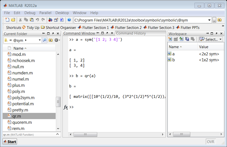
In a recent blog post, I demonstrated how to use the MATLAB 2012a Symbolic Toolbox to perform Variable precision QR decomposition in MATLAB. The result was a function called vpa_qr which did the necessary work.
>> a=vpa([2 1 3;-1 0 7; 0 -1 -1]);
>> [Q R]=vpa_qr(a);
I’ve suppressed the output because it’s so large but it definitely works. When I triumphantly presented this function to the user who requested it he was almost completely happy. What he really wanted, however, was for this to work:
>> a=vpa([2 1 3;-1 0 7; 0 -1 -1]);
>> [Q R]=qr(a);
In other words he wants to override the qr function such that it accepts variable precision types. MATLAB 2012a does not allow this:
>> a=vpa([2 1 3;-1 0 7; 0 -1 -1]);
>> [Q R]=qr(a)
Undefined function 'qr' for input arguments of type 'sym'.
I put something together that did the job for him but felt that it was unsatisfactory. So, I sent my code to The MathWorks and asked them if what I had done was sensible and if there were any better options. A MathWorks engineer called Hugo Carr sent me such a great, detailed reply that I asked if I could write it up as a blog post. Here is the result:
Approach 1: Define a new qr function, with a different name (such as vpa_qr). This is probably the safest and simplest option and was the method I used in the original blog post.
- Pros: The new function will not interfere with your MATLAB namespace
- Cons: MATLAB will only use this function if you explicitly define that you wish to use it in a given function. You would have to find all prior references to the qr algorithm and make a decision about which to use.
Approach 2: Define a new qr function and use the ‘isa’ function to catch instances of ‘sym’. This is the approach I took in the code I sent to The MathWorks.
function varargout = qr( varargin )

if nargin == 1 && isa( varargin{1}, 'sym' )
    [varargout{1:nargout}] = vpa_qr( varargin{:} );
else
    [varargout{1:nargout}] = builtin( 'qr', varargin{:} );
end
- Pros: qr will always select the correct code when executed on sym objects
- Cons: This code only works for shadowing built-ins and will produce a warning reminding you of this fact. If you wish to extend this pattern for other class types, you’ll require a switch statement (or nested if-then-else block), which could lead to a complex comparison each time qr is invoked (and subsequent performance hit). Note that switch statements in conjunction with calls to ‘isa’ are usually indicators that an object oriented approach is a better way forward.
Approach 3: The MathWorks do not recommend that you modify your MATLAB install. However for completeness, it is possible to add a new ‘method’ to the sym class by dropping your function into the sym class folder. For MATLAB 2012a on Windows, this folder is at
C:\Program Files\MATLAB\R2012a\toolbox\symbolic\symbolic\@sym
For the sake of illustration, here is a simplified implementation. Call it qr.m
function result = qr( this )
  result = feval(symengine,'linalg::factorQR', this);
end
Pros: Functions saved to a class folder take precedence over built in functionality, which means that MATLAB will always use your qr method for sym objects.
Cons: If you share code which uses this functionality, it won’t run on someone’s computer unless they update their sym class folder with your qr code. Additionally, if a new method is added to a class it may shadow the behaviour of other MATLAB functionality and lead to unexpected behaviour in Symbolic Toolbox.
Approach 4: For more of an object-oriented approach it is possible to sub-class the sym class, and add a new qr method.
classdef mySym < sym

    methods
        function this = mySym(arg)
            this = this@sym(arg);
        end

        function result = qr( this )
            result = feval(symengine,'linalg::factorQR', this);
        end
    end

end
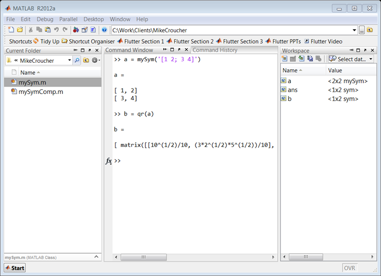
Pros: Your change can be shipped with your code and it will work on a client’s computer without having to change the sym class.
Cons: When calling superclass methods on your mySym objects (such as sin(mySym1)), the result will be returned as the superclass unless you explicitly redefine the method to return the subclass.
N.B. There is a lot of literature which discusses why inheritance (subclassing) to augment a class’s behaviour is a bad idea. For example, if Symbolic Toolbox developers decide to add their own qr method to the sym API, overriding that function with your own code could break the system. You would need to update your subclass every time the superclass is updated. This violates encapsulation, as the subclass implementation depends on the superclass. You can avoid problems like these by using composition instead of inheritance.
Approach 5: You can create a new sym class by using composition, but it takes a little longer than the other approaches. Essentially, this involves creating a wrapper which provides the functionality of the original class, as well as any new functions you are interested in.
classdef mySymComp

    properties
        SymProp
    end

    methods
        function this = mySymComp(symInput)
            this.SymProp = symInput;
        end

        function result = qr( this )
            result = feval(symengine,'linalg::factorQR', this.SymProp);
        end
    end

end
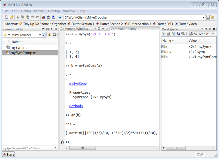
Note that in this example we did not add any of the original sym functions to the mySymComp class, however this can be done for as many as you like. For example, I might like to use the sin method from the original sym class, so I can just delegate to the methods of the sym object that I passed in during construction:
classdef mySymComp

    properties
        SymProp
    end

    methods
        function this = mySymComp(symInput)
            this.SymProp = symInput;
        end

        function result = qr( this )
            result = feval(symengine,'linalg::factorQR', this.SymProp);
        end

        function G = sin(this)
            G = mySymComp(sin(this.SymProp));
        end
    end

end
Pros: The change is totally encapsulated, and cannot be broken save for a significant change to the sym api (for example, the MathWorks adding a qr method to sym would not break your code).
Cons: The wrapper can be time consuming to write, and the resulting object is not a ‘sym’, meaning that if you pass a mySymComp object ‘a’ into the following code:
isa(a, 'sym')
MATLAB will return ‘false’ by default.
R has a citation() command that recommends how to cite the use of R in your publications, information that is also included in R’s Frequently Asked Questions document.
To cite R in publications use:

  R Core Team (2012). R: A language and environment for
  statistical computing. R Foundation for Statistical
  Computing, Vienna, Austria. ISBN 3-900051-07-0, URL
  http://www.R-project.org/.

A BibTeX entry for LaTeX users is

  @Manual{,
    title = {R: A Language and Environment for Statistical Computing},
    author = {{R Core Team}},
    organization = {R Foundation for Statistical Computing},
    address = {Vienna, Austria},
    year = {2012},
    note = {{ISBN} 3-900051-07-0},
    url = {http://www.R-project.org/},
  }

We have invested a lot of time and effort in creating R, please
cite it when using it for data analysis. See also
‘citation("pkgname")’ for citing R packages
This led me to wonder how often people cite the software they use. For example, if you publish the results of a simulation written in MATLAB do you cite MATLAB in any way? How about if you used Origin or Excel to produce a curve fit, would you cite that? Would you cite your plotting software, numerical libraries or even compiler?
The software sustainability institute (SSI), of which I recently became a fellow, has guidelines on how to cite software.
xkcd is a popular webcomic that sometimes includes hand drawn graphs in a distinctive style. Here’s a typical example

In a recent Mathematica StackExchange question, someone asked how such graphs could be automatically produced in Mathematica and code was quickly whipped up by the community. Since then, various individuals and communities have developed code to do the same thing in a range of languages. Here’s the list of examples I’ve found so far
- xkcd style graphs in Mathematica. There is also a Wolfram blog post on this subject.
- xkcd style graphs in R. A follow up blog post at vistat.
- xkcd style graphs in LaTeX
- xkcd style graphs in Python using matplotlib
- xkcd style graphs in MATLAB. There is now some code on the File Exchange that does this with your own plots.
- xkcd style graphs in javascript using D3
- xkcd style graphs in Euler
- xkcd style graphs in Fortran
Any I’ve missed?