
Archive for the ‘matlab’ Category
One of the new features in MATLAB 2010b that’s getting me very excited is the CUDA based GP-GPU (General Purpose computation on Graphical Processing Units) integration that’s become available in the Parallel Computing Toolbox. As soon as I had MATLAB 2010b installed on my CUDA capable laptop (Dell XPS M1330 with a GeForce 8400M GS) running Ubuntu I wanted to try out as much of this new functionality as my low-end hardware would allow me. I’ve installed and played with CUDA on this machine in the past and so I fired up MATLAB 2010b and issued the following command to ask MATLAB how many CUDA enabled devices it thought I had on my system
gpuDeviceCount

??? Error using ==> feval
The CUDA driver was found, but it is too old. The CUDA driver on your system is version: 3.
The required CUDA version is: 3.1 or greater.
The practical upshot of the above error message is that I needed to upgrade my NVidia graphics driver which was at version 195.36.24. I went for the latest version which, at the time of writing, is version 256.53. I did this from the NVIDIA-Linux-x86-256.53.run file which I got direct from NVidia and all I’ll say about the process is that it ruined an otherwise perfectly good Sunday morning. I did get there in the end though!
So, I had the shiniest version of the graphics driver up and running. Time to fire up MATLAB again:
>> gpuDeviceCount
Warning: The device selected (device 1, "GeForce 8400M
GS") does not have sufficient compute capability to be
used. Compute capability 1.3 (or greater) is required,
the selected device has compute capability 1.1.
> In deviceCount at 7
  In GPUDevice.GPUDevice>GPUDevice.count at 27
  In gpuDeviceCount at 10
Or, to put it another way, “Please insert new laptop to continue.” With that, my MATLAB/CUDA experiments are brought to an end.
Can anyone recommend a reasonably priced laptop that contains a CUDA capable graphics card at compute level 1.3 or above?
Update (16th September 2010): Several people have emailed me to defend The Mathwork’s design decision so I’d like to make something very clear: I completely agree with The Matworks in their insistence on CUDA compute level 1.3 or above. As one correspondent pointed out, this ensures that not only does the hardware support double precision but it is also IEEE-compliant and IEEE-compliance is a good thing! This blog post was never meant to criticize The Mathworks over this, I wrote it partly to ensure that more people are aware of the requirements and partly because I needed to vent over the sudden obsolescence of my relatively new laptop.
The MATLAB function ranksum is part of MATLAB’s Statistics Toolbox. Like many organizations who use network licensing for MATLAB and its toolboxes, my employer, The University of Manchester, sometimes runs out of licenses for this toolbox which leads to following error message when you attempt to evaluate ranksum.
??? License checkout failed.
License Manager Error -4
Maximum number of users for Statistics_Toolbox reached.
Try again later.
To see a list of current users use the lmstat utility or contact your License Administrator.
An alternative to the Statistics Toolbox is the NAG Toolbox for MATLAB for which we have an unlimited number of licenses. Here’s how to replace ranksum with the NAG routine g08ah.
Original MATLAB / Statistics Toolbox code
x = [0.8147;0.9058;0.1270;0.9134;0.6324;0.0975;0.2785;0.5469;0.9575;0.9649];
y=  [0.4076;1.220;1.207;0.735;1.0502;0.3918;0.671;1.165;1.0422;1.2094;0.9057;0.285;1.099;1.18;0.928];
p = ranksum(x,y)
The result is p = 0.0375
Code using the NAG Toolbox for MATLAB
x = [0.8147;0.9058;0.1270;0.9134;0.6324;0.0975;0.2785;0.5469;0.9575;0.9649];
y =  [0.4076;1.220;1.207;0.735;1.0502;0.3918;0.671;1.165;1.0422;1.2094;0.9057;0.285;1.099;1.18;0.928];
tail = 'T';
[u, unor, p, ties, ranks, ifail] = g08ah(x, y, tail);
The value for p is the same as that calculated by ranksum: p = 0.0375
NAG’s g08ah routine returns a lot more than just the value p but, for this particular example, we can just ignore it all. In fact, if you have MATLAB 2009b or above then you could call g08ah like this
tail = 'T';
[~, ~, p, ~, ~, ~] = g08ah(x, y, tail);
Which explicitly indicates that you are not going to use any of the outputs other than p.
People at Manchester are using the NAG toolbox for MATLAB more and more; not only because we have a full site license for it but because it can sometimes be very fast. Here’s some more articles on the NAG toolbox you may find useful.
A bit of background to this post
I work in the IT department of the University of Manchester and we are currently developing a Condor Pool which is basically a method of linking together hundreds of desktop machines to produce a high-throughput computing resource. A MATLAB user recently submitted some jobs to our pool and complained that all of them gave identical results which is stupid because his code used MATLAB’s rand command to mix things up a bit.
I was asked if I knew why this should happen to which I replied ‘yes.’ I was then asked to advise the user how to fix the problem and I did so. The next request was for me to write some recommendations and tutorials on how users should use random numbers in MATLAB (and Mathematica and possibly Python while I was at it) along with our Condor Pool and I went uncharacteristically quiet for a while.
It turned out that I had a lot to learn about random numbers. This is the first of a series of (probably 2) posts that will start off by telling you what I knew and move on to what I have learned. It’s as much a vehicle for getting the concepts straight in my head as it is a tutorial.
Ask MATLAB for 10 Random Numbers
Before we go on, I’d like you to try something for me. You have to start on a system that doesn’t have MATLAB running at all so if MATLAB is running then close it before proceeding. Now, open up MATLAB and before you do anything else issue the following command
rand(10,1)
As many of you will know, the rand command produces random numbers from the uniform distribution between 0 and 1 and the command above is asking for 10 such numbers. You may reasonably expect that the 10 random numbers that you get will be different from the 10 random numbers that I get; after all, they are random right? Well, I got the following numbers when running the above command on MATLAB 2009b running on Linux.
ans =
0.8147
0.9058
0.1270
0.9134
0.6324
0.0975
0.2785
0.5469
0.9575
0.9649
Look familiar?
Now I’ve done this experiment with a number of people over the last few weeks and the responses can be roughly split into two different camps as follows:
1. Oh yeah, I know all about that – nothing to worry about. It’s pretty obvious why it happens isn’t it?
2. It’s a bug. How can the numbers be random if MATLAB always returns the same set?
What does random mean anyway?
If you are new to the computer generation of random numbers then there is something that you need to understand and that is that, strictly speaking, these numbers (like all software generated ‘random’ numbers) are not ‘truly’ random. Instead they are pseudorandom – my personal working definition of which is “A sequence of numbers generated by some deterministic algorithm in such a way that they have the same statistical properties of ‘true’ random numbers”. In other words, they are not random they just appear to be but the appearance is good enough most of the time.
Pseudorandom numbers are generated from deterministic algorithms with names like Mersenne Twister, L’Ecuyer’s mrg32k3a [1] and Blum Blum Schub whereas ‘true’ random numbers come from physical processes such as radioactive decay or atmospheric noise (the website www.random.org uses atmospheric noise for example).
For many applications, the distinction between ‘truly random’ and ‘pseudorandom’ doesn’t really matter since pseudorandom numbers are ‘random enough’ for most purposes. What does ‘random enough’ mean you might ask? Well as far as I am concerned it means that the random number generator in question has passed a set of well defined tests for randomness – something like Marsaglia’s Diehard tests or, better still, L’Ecuyer and Simard’s TestU01 suite will do nicely for example.
The generation of random numbers is a complicated topic and I don’t know enough about it to do it real justice but I know a man who does. So, if you want to know more about the theory behind random numbers then I suggest that you read Pierre L’Ecuyer’s paper simply called ‘Random Numbers’ (pdf file).
Back to MATLAB…
Always the same seed
So, which of my two groups are correct? Is there a bug in MATLAB’s random number generator or not?
There is nothing wrong with MATLAB’s random number generator at all. The reason why the command rand(10,1) will always return the same 10 numbers if executed on startup is because MATLAB always uses the same seed for its pseudorandom number generator (which at the time of writing is a Mersenne Twister) unless you tell it to do otherwise.
Without going into details, a seed is (usually) an integer that determines the internal state of a random number generator. So, if you initialize a random number generator with the same seed then you’ll always get the same sequence of numbers and that’s what we are seeing in the example above.
Sometimes, this behaviour isn’t what we want. For example, say I am doing a Monte Carlo simulation and I want to run it several times to verify my results. I’m going to want a different sequence of random numbers each time or the whole exercise is going to be pointless.
One way to do this is to initialize the random number generator with a different seed at startup and a common way of achieving this is via the system clock. The following comes straight out of the current MATLAB documentation for example
RandStream.setDefaultStream(RandStream('mt19937ar','seed',sum(100*clock)));
If you are using MATLAB 2011a or above then you can use the following, much simpler syntax to do the same thing
rng shuffle
Do this once per MATLAB session and you should be good to go (there is usually no point in doing it more than once per session by the way….your numbers won’t be any ‘more random’ if you so. In fact, there is a chance that they will become less so!).
Condor and ‘random’ random seeds
Sometimes the system clock approach isn’t good enough either. For example, at my workplace, Manchester University, we have a Condor Pool of hundreds of desktop machines which is perfect for people doing Monte Carlo simulations. Say a single simulation takes 5 hours and it needs to be run 100 times in order to get good results. On one machine that’s going to take about 3 weeks but on our Condor Pool it can take just 5 hours since all 100 simulations run at the same time but on different machines.
If you don’t think about random seeding at all then you end up with 100 identical sets of results using MATLAB on Condor for the reasons I’ve explained above. Of course you know all about this so you switch to using the clock seeding method, try again and….get 100 identical sets of results[2].
The reason for this is that the time on all 100 machines is synchronized using internet time servers. So, when you start up 100 simultaneous jobs they’ll all have the same timestamp and, therefore, have the same random seed.
It seems that what we need to do is to guarantee (as far as possible) that every single one of our condor jobs gets a unique seed in order to provide a unique random number stream and one way to do this would be to incorporate the condor process ID into the seed generation in some way and there are many ways one could do this. Here, however, I’m going to take a different route.
On Linux machines it is possible to obtain small numbers of random numbers using the special files /dev/random and /dev/urandom which are interfaces to the kernel’s random number generator. According to the documentation ‘The random number generator gathers environmental noise from device drivers and other sources into an entropy pool. The generator also keeps an estimate of the number of bit of the noise in the entropy pool. From this entropy pool random numbers are created.’
This kernel generator isn’t suitable for simulation purposes but it will do just fine for generating an initial seed for MATLAB’s pseudorandom number generator. Here’re the MATLAB commands
[status seed] = system('od /dev/urandom --read-bytes=4 -tu | awk ''{print $2}''');
seed=str2double(seed);
RandStream.setDefaultStream(RandStream('mt19937ar','seed',seed));
In MATLAB 2011a or above you can change this to
[status seed] = system('od /dev/urandom --read-bytes=4 -tu | awk ''{print $2}''');
seed=str2double(seed);
rng(seed);
Put this at the beginning of the MATLAB script that defines your condor job and you should be good to go. Don’t do it more than once per MATLAB session though – you won’t gain anything!
The end or the end of the beginning?
If you asked me the question ‘How do I generate a random seed for a pseudorandom number generator?’ then I think that the above solution answers it quite well. If, however, you asked me ‘What is the best way to generate multiple independent random number streams that would be good for thousands of monte-carlo simulations?‘ then we need to rethink somewhat for the following reasons.
Seed collisions: The Mersenne twister algorithm currently used as the default random number generator for MATLAB uses a 32bit integer seed which means that it can take on 2^32 or 4,294,967,296 different values – which seems a lot! However, by considering a generalisation of the birthday problem it can be seen that if you select such a seed at random then you have a 50% chance choosing two identical seeds after only 65,536 runs. In other words, if you perform 65,536 simulations then there is a 50% chance that two such simulations will produce identical results.
Bad seeds: I have read about (but never experienced) the possibility of ‘bad seeds’; that is some seeds that produce some very strange, non-random results – for the first few thousand iterates at least. This has led to some people advising that you should ‘warm-up’ your random number generator by asking for, and throwing away, a few thousand random numbers before you start using them. Does anyone know of any such bad seeds?
Overlapping or correlated sequences: All pseudorandom number generators are periodic (at least, all the ones that I know about are) – which means that after N iterations the sequence repeats itself. If your generator is good then N is usually large enough that you don’t need to worry about this. The Mersenne Twister used in MATLAB, for instance, has a huge period of (2^19937 – 1)/2 (half of the standard 32bit implementation).
The point I want to make is that you don’t get several different streams of random numbers, you get just one, albeit a very big one. Now, when you choose a seed you are essentially choosing a random point in this stream and there is no guarantee how far apart these two points are. They could be separated by a distance of trillions of points or they could be right next to each other – we simply do not know – and this leads to the possibility of overlapping sequences.
Now, one could argue that the possibility of overlap is very small in a generator such as the Mersenne Twister and I do not know of any situation where it has occurred in practice but that doesn’t mean that we shouldn’t worry about it. If your work is based on the assumption that all of your simulations have used independent, uncorrelated random number streams then there is a possibility that your assumptions could be wrong which means that your conclusions could be wrong. Unlikely maybe, but still no way to do science.
Next Time
Next time I’ll be looking at methods for generating guaranteed independent random number streams using MATLAB’s in-built functions as well as methods taken from the NAG Toolbox for MATLAB. I’ll also be including explicit examples that use this stuff in Condor.
Ask the audience
I assume that some of you will be in the business of performing Monte-Carlo simulations and so you’ll probably know much more about all of this than me. I have some questions
- Has anyone come across any ‘bad seeds’ when dealing with MATLAB’s Mersenne Twister implementation?
- Has anyone come across overlapping sequences when using MATLAB’s Mersenne Twister implementation?
- How do YOU set up your random number generator(s).
I’m going to change my comment policy for this particular post in that I am not going to allow (most) anonymous comments. This means that you will have to give me your email address (which, of course, I will not publish) which I will use once to verify that it really was you that sent the comment.
Notes and References
[1] L’Ecuyer P (1999) Good parameter sets for combined multiple recursive random number generators Operations Research 47:1 159–164
[2] More usually you’ll get several different groups of results. For example you might get 3 sets of results, A B C, and get 30 sets of A, 50 sets of B and 20 sets of C. This is due to the fact that all 100 jobs won’t hit the pool at precisely the same instant.
[3] Much of this stuff has already been discussed by The Mathworks and there is an excellent set of articles over at Loren Shure’s blog – Loren onThe Art of MATLAB.
MATLAB contains a function called pdist that calculates the ‘Pairwise distance between pairs of objects’. Typical usage is
X=rand(10,2);
dists=pdist(X,'euclidean');
It’s a nice function but the problem with it is that it is part of the Statistics Toolbox and that costs extra. I was recently approached by a user who needed access to the pdist function but all of the statistics toolbox license tokens on our network were in use and this led to the error message
??? License checkout failed.
License Manager Error -4
Maximum number of users for Statistics_Toolbox reached.
Try again later.
To see a list of current users use the lmstat utility or contact your License Administrator
One option, of course, is to buy more licenses for the statistics toolbox but there is another way. You may have heard of GNU Octave, a free,open-source MATLAB-like program that has been in development for many years. Well, Octave has a sister project called Octave-Forge which aims to provide a set of free toolboxes for Octave. It turns out that not only does Octave-forge contain a statistics toolbox but that toolbox contains an pdist function. I wondered how hard it would be to take Octave-forge’s pdist function and modify it so that it ran on MATLAB.
Not very! There is a script called oct2mat that is designed to automate some of the translation but I chose not to use it – I prefer to get my hands dirty you see. I named the resulting function octave_pdist to help clearly identify the fact that you are using an Octave function rather than a MATLAB function. This may matter if one or the other turns out to have bugs. It appears to work rather nicely:
dists_oct = octave_pdist(X,'euclidean');
% let's see if it agrees with the stats toolbox version
all( abs(dists_oct-dists)<1e-10)

ans =
     1
Let’s look at timings on a slightly bigger problem.
>> X=rand(1000,2);
>> tic;matdists=pdist(X,'euclidean');toc
Elapsed time is 0.018972 seconds.
>> tic;octdists=octave_pdist(X,'euclidean');toc
Elapsed time is 6.644317 seconds.
Uh-oh! The Octave version is 350 times slower (for this problem) than the MATLAB version. Ouch! As far as I can tell, this isn’t down to my dodgy porting efforts, the original Octave pdist really does take that long on my machine (Ubuntu 9.10, Octave 3.0.5).
This was far too slow to be of practical use and we didn’t want to be modifying algorithms so we ditched this function and went with the NAG Toolbox for MATLAB instead (routine g03ea in case you are interested) since Manchester effectively has an infinite number of licenses for that product.
If,however, you’d like to play with my MATLAB port of Octave’s pdist then download it below.
- octave_pdist.m makes use of some functions in the excellent NaN Toolbox so you will need to download and install that package first.
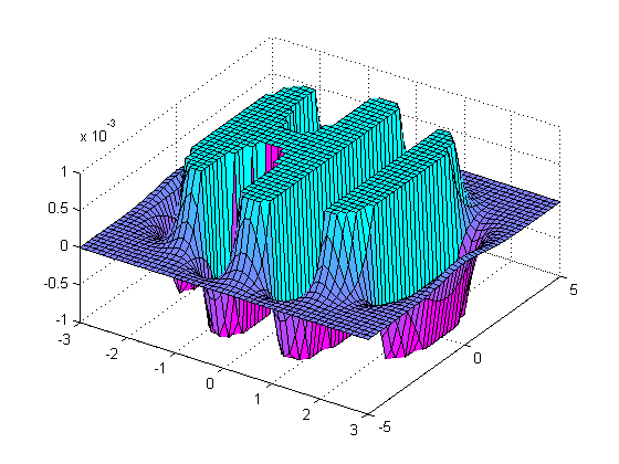
One of the earliest posts I made on Walking Randomly (almost 3 years ago now – how time flies!) described the following equation and gave a plot of it in Mathematica.


Some time later I followed this up with another blog post and a Wolfram Demonstration.
Well, over at Stack Overflow, some people have been rendering this cool equation using MATLAB. Here’s the first version
x = linspace(-3,3,50);
y = linspace(-5,5,50);
[X Y]=meshgrid(x,y);
Z = exp(-X.^2-Y.^2/2).*cos(4*X) + exp(-3*((X+0.5).^2+Y.^2/2));
Z(Z>0.001)=0.001;
Z(Z<-0.001)=-0.001;
surf(X,Y,Z);
colormap(flipud(cool))
view([1 -1.5 2])
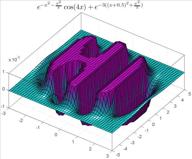
and here’s the second.
[x y] = meshgrid( linspace(-3,3,50), linspace(-5,5,50) );
z = exp(-x.^2-0.5*y.^2).*cos(4*x) + exp(-3*((x+0.5).^2+0.5*y.^2));
idx = ( abs(z)>0.001 );
z(idx) = 0.001 * sign(z(idx));

figure('renderer','opengl')
patch(surf2patch(surf(x,y,z)), 'FaceColor','interp');
set(gca, 'Box','on', ...
    'XColor',[.3 .3 .3], 'YColor',[.3 .3 .3], 'ZColor',[.3 .3 .3], 'FontSize',8)
title('$e^{-x^2 - \frac{y^2}{2}}\cos(4x) + e^{-3((x+0.5)^2+\frac{y^2}{2})}$', ...
    'Interpreter','latex', 'FontSize',12)

view(35,65)
colormap( [flipud(cool);cool] )
camlight headlight, lighting phong
Do you have any cool graphs to share?
The Mathworks have released a new app for iPhone and iPad called MATLAB Mobile. When I first saw the headlines I was very excited but the product is rather disappointing in my opinion since all it does is offer a mobile interface to an instance of MATLAB running on a desktop machine. While this might be useful to some people I have to admit that it doesn’t light any fires for me. I’ll save my excitement for a mobile MATLAB application that can actually do some mathematics locally.
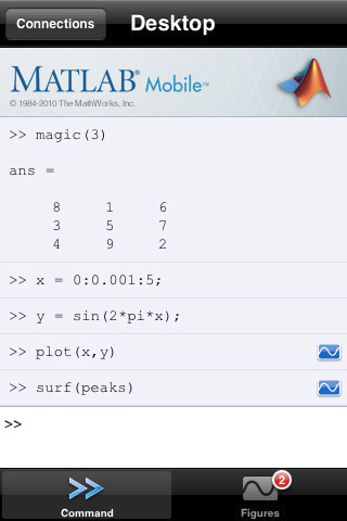
How about you though? Will this new application be useful for the way you work?
More articles from Walking Randomly on mobile mathematics software
Reading comma separated value (csv) files into MATLAB is trivial as long as the csv file you are trying to import is trivial. For example, say you wanted to import the file very_clean.txt which contains the following data
1031,-948,-76
507,635,-1148
-1031,948,750
-507,-635,114
The following, very simple command, is all that you need
>> veryclean = csvread('very_clean.txt')

veryclean =

        1031        -948         -76
         507         635       -1148
       -1031         948         750
        -507        -635         114
In the real world, however, your data is rarely this nice and clean. One of the most common problems faced by MATLABing data importers is that of header lines. Take the file quite_clean.txt for instance. This is identical to the previous example apart from the fact that it contains two header lines
These are some data that I made using my hand-crafted code
Date:12th July 1996
1031,-948,-76
507,635,-1148
-1031,948,750
-507,-635,114
This is all too much for the csvread command
>> data=csvread('quite_clean.txt')
??? Error using ==> dlmread at 145
Mismatch between file and format string.
Trouble reading number from file (row 1, field 1) ==> This

Error in ==> csvread at 52
    m=dlmread(filename, ',', r, c);
Not to worry, we can just use the more capable importdata command instead
>> quiteclean = importdata('quite_clean.txt')

quiteclean =

        data: [4x3 double]
    textdata: {2x1 cell}
The result above is a two element structure array and our numerical values are contained in a field called data. Here’s how you get at it.
>> quiteclean.data

ans =

        1031        -948         -76
         507         635       -1148
       -1031         948         750
        -507        -635         114
So far so good. How do we handle a file like messy_data.txt though?
header 1;
header 2;
1031,-948,-76, ,"12"
507,635,-1148, ,"34"
-1031,948,750, ,"45"
-507,-635,114, ,"67"
This is the kind of file encountered by Walking Randomly reader ‘reen’ and it contains exactly the same numerical values as the previous two examples. Unfortunately, it also contains some cruft that makes life more difficult for us. Let’s bring out the big-guns!
Using textscan to import csv files in MATLAB
When the going gets tough, the tough use textscan. Here’s the incantation for importing messy_data.txt
fid=fopen('messy_data.txt');
data = textscan(fid,'%f %f %f %*s %*s','HeaderLines',2,'Delimiter',',','CollectOutput',1);
fclose(fid)
The result is a one-element cell array that contains an array of doubles. Let’s get the array of doubles out of the cell
>> data=data{1}
data =
        1031        -948         -76
         507         635       -1148
       -1031         948         750
        -507        -635         114
If the importdata command is a chauffeur then textscan is a Ferrari and I don’t know about you but I’d much rather be driving my own Ferrari than being chauffeured around (John Cook over at The Endeavour has more to say on Ferraris and Chauffeurs).
Let’s de-construct the above set of commands. The first thing to notice is that, unlike csvread and importdata, you have to explicitly open and close your file when using the textscan command. So, you open your file using fopen and give it a file ID (which in this example is fid).
fid=fopen('messy_data.txt');
The first argument to textscan is just this file ID, fid. Next you need to supply a conversion specifier which in this case is
'%f %f %f %*s %*s'
The conversion specifier tells textscan what you want each row in your csv file to be converted to. %f means “64 bit double” and %s means “string” so ‘%f %f %f %s %s’ means “3 doubles followed by 2 strings” (we’ll get onto the asterisks in the original specifier later). You can use all sorts of data types in a conversion specifier such as integers, quoted strings and pattern matched strings among others. Check out the MATLAB documentation for textscan for the full list but an abbreviated list is shown below:
%d signed 32bit integer
%u unsigned 32bit integer
%f 64bit double (you'll want this most of the time when using MATLAB)
%s string
Now, in the command I used to import messy_data.txt the conversion specifier contained some asterisks such as %*s so what do these mean? Quite simply, the asterisk just means ‘ignore’ so %*s means ‘ignore the string in this field’. So, the full meaning of my conversion specifier ‘%f %f %f %*s %*s’ is “read 3 doubles and ignore 2 strings” and textscan will do this for every row.
The rest of the command is pretty self explanatory but I’ll explain it anyway for the sake of completeness
'HeaderLines',2
The file has 2 headerlines which should be ignored
'Delimiter',','
The fields are delimited (a posh word for separated) by a comma
'CollectOutput',1
If you supply a 1 (which stands for True) to the CollectOutput option then textscan will join consecutive output cells with the same data type into a single array. Since I want all of my doubles to be in a single array then this is the behaviour I went for.
Finally, once you have finished textscanning, don’t forget to close your file
fclose(fid)
That’s pretty much it for this mini-tutorial – I hope you find it useful.
I have got a nice, shiny 64bit version of MATLAB running on my nice, shiny 64bit Linux machine and so, naturally, I wanted to be able to use 64 bit integers when the need arose. Sadly, MATLAB had other ideas. On MATLAB 2010a:
a=int64(10);
b=int64(20);
a+b
??? Undefined function or method 'plus' for input arguments of type 'int64'.
It doesn’t like any of the other operators either
>> a-b
??? Undefined function or method 'minus' for input arguments of type 'int64'.

>> a*b
??? Undefined function or method 'mtimes' for input arguments of type 'int64'.

>> a/b
??? Undefined function or method 'mrdivide' for input arguments of type 'int64'.
At first I thought that there was something wrong with my MATLAB installation but it turns out that this behaviour is expected and documented. At the time of writing, the MATLAB documentation contains the lines
Note   Only the lower order integer data types support math operations.
Math operations are not supported for int64 and uint64.
So, there you have it. When can’t MATLAB add up? When you ask it to add 64 bit integers!
Update: Just had an email from someone who points out that Octave (Free MATLAB Clone) can handle 64bit integers just fine
octave:1> a=int64(10);
octave:2> b=int64(20);
octave:3> a+b
ans = 30
octave:4>
Update 2: Since I got slashdotted, people have been asking why I (or, more importantly, the user I was helping) needed 64bit integers. Well, we were using the NAG Toolbox for MATLAB which is a MATLAB interface to the NAG Fortran library. Some of its routines require integer arguments and on a 64bit machine these must be 64bit integers. We just needed to do some basic arithmetic on them before passing them to the toolbox and discovered that we couldn’t. The work-around was simple – use int32s for the arithmetic and then convert to int64 at the end so no big deal really. I was simply surprised that arithmetic wasn’t supported for int64s directly – hence this post.
Update 3: In the comments, someone pointed out that there is a package on the File Exchange that adds basic arithmetic support for 64bit integers. I’ve not tried it myself though so can’t comment on its quality.
Update 4: Someone has made me aware of an interesting discussion concerning this topic on MATLAB Central a few years back: http://www.mathworks.com/matlabcentral/newsreader/view_thread/154955
Update 5 (14th September 2010): MATLAB 2010b now has support for 64 bit integers.
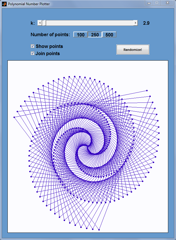
After reading my recent post, Polygonal numbers on quadratic number spirals, Walking Randomly reader Matt Tearle came up with a MATLAB version and it looks great. Click on the image below for the code.
The latest version of MATLAB – MATLAB 2010a – was released on Friday 5th March. As always, the full list of changes is extensive but some of the highlights from my point of view include the following.
Bug Fixes
MATLAB 2009b contained bugs in some core pieces of functionality. I am now very happy to report that these have been fixed.
- A serious bug in MATLAB 2009b fixed in 2010a
- A bug in the sort function that affected arrays of complex numbers on some platforms. Fixed in 2010a
Parallel and Multicore enhancements
Almost everyone has a multicore processor these days and they expect programs such as MATLAB to take full advantage of them. However, parallel programming can be hard work and so it is impossible to make every function become ‘multicore aware’ overnight. Almost every release of MATLAB gives us a few more functions that make use of our new multicore processors.
- Multicore support for several functions from the image processing toolbox. I’ve added these to my list of known ‘multicore aware’ functions in MATLAB.
- The Fast Fourier Transform function – fft – was originally made multicore-aware back in release 2009a and this has been improved on in 2010a. The multithreaded improvements for fft in 2009a were for multichannel Fast Fourier Transforms. In other words, when taking the FFT of a 2D array, MATLAB computes the FFT of each column on an independent thread. The improvements in 2010a actually multithread the calculation of a single FFT. Mathworks refer to this as “long vector” FFT since this speeds up the calculations of a very long fft.
Other articles you may be interested in on parallel programming in MATLAB.
- Parallel MATLAB with openmp mex files
- Parallelisation: Is MATLAB doing it wrong?
- Supercharge MATLAB with your graphics card
- A list of multicore functions in MATLAB
Changes to the symbolic toolbox
The symbolic toolbox for MATLAB is one of my favourite Mathworks products since it offers so much extra functionality. Most toolboxes are just a set of .m MATLAB files but the symbolic toolbox includes an entire program called MUPAD along with a set of interfaces to MATLAB itself. Lets look at some of the enhancements developed in 2010a in detail.
- MuPAD demonstrates better performance when handling some linear algebra operations on matrices containing symbolic elements. Let’s look at symbolic Matrix Inversion for example. Take the following piece of MUPAD code
x:= 1 + sin(a) + cos(b):
A:= matrix( [ [11/x + a11, 12/x + a12, 13/x + a13, 14/x + a14],
              [21/x + a21, 22/x + a22, 23/x + a23, 24/x + a24],
              [31/x + a31, 32/x + a32, 33/x + a33, 34/x + a34],
              [41/x + a41, 42/x + a42, 43/x + a43, 44/x + a44] ]):
time((B:= 1/A))*sec/1000.0;
On my machine, 2009a did this calculation in 61.1 seconds whereas 2010a did it in 0.9 seconds. That’s one heck of a speedup!
- Enhanced simplification functions, simplify and Simplify, demonstrate better results for expressions involving trigonometric and hyperbolic functions, square roots, and sums over roots of unity. There’s a lot of improvements packed into this one bullet point but I’ll just focus on one particular example. Take the following MUPAD code.
f:= -( ((x + 1)^(1/2) - 1)
      *((1 - x)^(1/2) - 1)*(4*x*(x + 1)^(1/2) + 8*(1 - x)^(1/2)*(x + 1)^(1/2) + 4*(x + 1)^(1/2)
     + 12*(x + 1)^(3/2) - 4*x*(1 - x)^(1/2) + 4*(1 - x)^(1/2) + 12*(1 - x)^(3/2) - 8*x^2 - 40)
     ) /(6*((x + 1)^(1/2) + (1 - x)^(1/2) - 2)^3)
     - (1/3*(x + 1)^(3/2) + 1/3*(1 - x)^(3/2)):
simplify(f)
If you evaluate this in the MUPAD notebook of release 2009b then you get a big mess. Evaluating it in 2010a, on the other hand, results in 0. Much tidier!
- Polynomial division has improved functionality. In R2009b it was not possible to divide multivariate polynomials with remainder,only exact division was possible. R2010a returns the quotient and the remainder. Consider the following MUPAD code.
q := poly(x+y^2+1):
p := poly(x^2+y)*q + poly(y^3+x)*q + poly(x^2+y^2+1):
divide(p, q);
2009b MUPAD just gives an error message
Error: Illegal argument [divide]
2010a,on the other hand, gives us what we want returning the quotient and the remainder.
poly(x^2 + 2*x + y^3 - y^2 + y - 1, [x, y]), poly(y^4 + 3*y^2 + 2, [x, y])
- The symbolic ODE solver in MUPAD now handles many more equation types. Here’s a particular example of a 2nd order linear ODE with hypergeometric solutions that can now be solved.
eq:= x^2*(x^2+1)*diff(y(x),x,x)+x*(2*x^2+1)*diff(y(x),x)-(nu*(nu+1)*x^2+n^2)*y(x);
solve(ode(eq,y(x)))
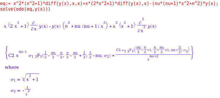
This is just a small selection of the enhancements that The Mathworks have made to the symbolic toolbox which is coming along in leaps and bounds in my humble opinion. Thanks to various members of staff at The Mathworks for supplying me with these examples (and a fair few more besides). I wouldn’t have been able to make this post without them.
Other articles on Walking Randomly about the symbolic toolbox for MATLAB:
- Review of the new symbolic toolbox in MATLAB 2008b (written just after the transfer from a Maple symbolic engine to the new Mupad one)
Changes to the Optimization toolbox
- The fmincon function now has a new algorithm available. The algorithm is called SQP which stands for Sequential Quadratic Programming. I don’t know much about it yet but may return to this in the future.
Licensing changes
Licensing and toolbox naming might be dull for most people – but it is a big deal to me since I work in a team that administers a large network license for MATLAB. Changes that might seem minor to most people can result in drastic improvements for the life of a network license administrator. On the other hand, some changes can result in massive amounts of work.
- Solaris as a network license platform was dropped. This is a shame because although my employer has very few Solaris client machines, it currently runs its MATLAB license server on Solaris and it has been (and continues to be) rock solid. Now we are going to have to move to Windows license servers and update every single client machine on campus before we can update to 2010a. Oh joys!
- The Genetic Algorithm and Direct Search toolbox is no more. It’s functionality is now part of the Global Optimization Toolbox. I’ve not used this one myself yet but it does have a small core set of users at my university.
Articles aimed at users of MATLAB network licenses include
- More MATLAB statistics toolbox licensing woes (and how to solve them)
- An alternative to binopdf using the NAG toolbox for MATLAB
Much of the fine detail in this article was provided to me by members of staff at The Mathworks. I thank them all for their time, patience and expertise in answering my incessant questions. Any mistakes, however, are my fault!
If you enjoyed this article, feel free to click here to subscribe to my RSS Feed.