
Archive for the ‘matlab’ Category
My passions include mathematics, mathematical software and gadgets. So, I instantly fell in love with the LED Cube. The programming was done in C but MATLAB was used for some of the prototyping.
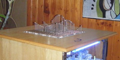
If you prefer something more physical then how about the MATLAB-controlled 3D function machine?
Perhaps you prefer a more retro, aural kind of a vibe? MATLAB-controlled carol singing dot-matrix printers anyone?
Update: In case it isn’t clear. None of the three projects above are my work, they are other people’s work! I just think they are cool!
Want to have a play?
If you’d like to use MATLAB as a way into physical computing then maybe the following resources will help you. I don’t think that they were used in the projects above but if I were to start playing with such things then I probably begin with one of these.
MATLAB’s control system toolbox has functions for converting transfer functions to either state space representations or zero-pole-gain models as follows
%Create a simple transfer function in MATLAB
num=[2 3];
den = [1 4 0 5];
mytf=tf(num,den);

%convert this to State Space form
tf2ss(num,den)
ans =

0   1   0
0   0   1
-5  -0  -4

%Convert to zero-pole-gain form
[z,p,k]=tf2zp(num,den)
z = -1.5000
p =

-4.27375 + 0.00000i
0.13687 + 1.07294i
0.13687 - 1.07294i

k =  2
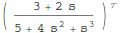
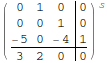
Now that Mathematica 8 is available I wondered what the Mathematica equivalent to the above would look like. The conversion to a StateSpace model is easy:
mytf=TransferFunctionModel[(2 s + 3)/(s^3 + 4 s^2 + 5), s]
StateSpaceModel[mytf]
but I couldn’t find an equivalent to MATLAB’s tf2zp function.
I can get the poles and zeros easily enough (as an aside it’s nice that Mathematica can do this exactly)
TransferFunctionPoles[mytf]
TransferFunctionZeros[mytf]
but what about gain? There is no TransferFunctionGain[] function as you might expect. There is a TransferFunctionFactor[] function but that doesn’t do what I want either.
It turns out that there is a function that will do what I want but it is hidden from the user a little in an internal function
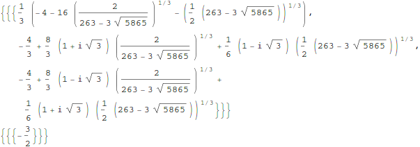
Control`ZeroPoleGainModel[mytf]

Control`ZeroPoleGainModel[{{{{-(3/2)}}}, {1/
     3 (-4 - 16 (2/(263 - 3 Sqrt[5865]))^(
        1/3) - (1/2 (263 - 3 Sqrt[5865]))^(1/3)), -(4/3) +
     8/3 (1 + I Sqrt[3]) (2/(263 - 3 Sqrt[5865]))^(1/3) +
     1/6 (1 - I Sqrt[3]) (1/2 (263 - 3 Sqrt[5865]))^(1/3), -(4/3) +
     8/3 (1 - I Sqrt[3]) (2/(263 - 3 Sqrt[5865]))^(1/3) +
     1/6 (1 + I Sqrt[3]) (1/2 (263 - 3 Sqrt[5865]))^(1/3)}, {{2}}}, s]
That’s not as user friendly as it could be though. How about this?
tf2zpk[x_] := Module[{z, p, k,zpkmodel},
  zpkmodel = Control`ZeroPoleGainModel[x];
  z = zpkmodel[[1, 1, 1, 1]];
  p = zpkmodel[[1, 2]];
  k = zpkmodel[[1, 3, 1]];
  {z, p, k}
  ]
Now we can get very similar behavior to MATLAB:
In[10]:= tf2zpk[mytf] // N

Out[10]= {{-1.5}, {-4.27375, 0.136874 + 1.07294 I,
  0.136874 - 1.07294 I}, {2.}}
Hope this helps someone out there. Thanks to my contact at Wolfram who told me about the Control`ZeroPoleGainModel function.
Other posts you may be interested in
MATLAB 2010b was released a couple of months ago and, as usual, it comes with a whole range of new features, performance enhancements and all important bug fixes. Within the MATLAB 2010b documentation, there are lists of the new functionality but I like to dig in a bit deeper and pick out one or two things that are of personal interest to me.
64 bit integer support
Back in April 2010, I was working with the NAG Toolbox for MATLAB which makes use of 64 bit integers on 64 bit machines and I learned that MATLAB 2010a and earlier didn’t support even the most basic of operations on 64 bit integers. For example, on MATLAB 2010a:
a=int64(10);
b=int64(20);
a+b
??? Undefined function or method 'plus' for input arguments of type 'int64'.
I’m happy to report that this has now been fixed and The Mathworks have implemented 18 basic operators for 64bit integer types including arithmetic, the colon operator, bsxfun and more. This has made my life (and the lives of some of the people I support) MUCH easier and I really appreciate The Mathworks work on this one.
Curve Fitting and Splines toolboxes merged
MATLAB has got a lot of toolboxes. In fact, it’s got far too many in my opinion which makes the product more expensive and fragmented. I have literally lost count of the amount of times someone has emailed me with a query like “I don’t suppose you have access to the XYZ toolbox because someone had sent me code that uses it and I can’t run it’ Quite frankly, it sucks.
So, when The Mathworks announce that they are merging the functionality of two related toolboxes into one, there is much rejoicing in Walking Randomly towers. If The Mathworks would like to do some more toolbox merging then I have a couple of suggestions :)
CUDA support in the Parallel Computing Toolbox
These days, the hotness in research computing is to do as much of your calculation as possible on your graphics card. If handled correctly, the hunk of silicon that was originally designed to make games look pretty can speed up scientific calculations hundreds of times compared to dull old CPUs. There is a great deal of interest in GP-GPU programming at Manchester University (my employer), so much so that we have set up a GPU-Club for our researchers.
Arguably, the leader in GP-GPU (General Purpose – Graphics Processing Unit) hardware is NVIDIA who are the developers of the CUDA programming framework. Until now, CUDA support in MATLAB has been provided by third-parties such as Jacket (Commerical) or GP-You (free) but as of 2010b, there is now official support for CUDA GPUs in MATLAB’s parallel computing toolbox. At the moment, it is not as well developed as products such as Jacket but I would lay bets that this will change in the not too distant future.
My early experiments with this new functionality have met with zero success but I have new hardware on the way and I am really looking forward to getting my teeth into this.
Parallel Statistics
Parallel computing in MATLAB is more complicated than it should be. Some functions make use of multicore processors automatically and you don’t need the parallel computing toolbox to feel the benefit. On the other hand, there are an increasing number of functions in toolboxes such as statistics and optimisation, that additionally require the PCT in order to make maximum use of modern hardware.
The 2010b version of the statistics toolbox includes an extra 8 functions (candexch, cordexch, daugment, dcovary, nnmf, plsregress, rowexch and sequentialfs) that now make use of the PCT. If you have the PCT, then this is wonderful news but if you don’t then there is nothing to see here.
Faster trig functions when the argument is in degrees
The standard trigonometric functions such as sin, cos, tan and the like all work in radians but MATLAB also has several functions that accept their arguments in degrees: sind, cosd and tand for example. In MATLAB 2010b these functions have been made significantly faster. Lets see how much faster using my 3Ghz quad Core 2 Q9650 running Ubuntu 9.10
In MATLAB 2010a
x=rand(1,1000000)*360;
>> tic;y=cosd(x);toc
Elapsed time is 0.120207 seconds.
In MATLAB 2010b
x=rand(1,1000000)*360;
>> tic;y=cosd(x);toc
Elapsed time is 0.021256 seconds.
A speed up of around 5.6 times! What’s more, I’ve already come across a user’s code in the wild where this optimisation made a real difference to their execution time. As far as I can tell, the speed up comes from the fact that 2010a and below uses MATLAB code for these functions whereas 2010b and above uses mex files.
What other bloggers say about MATLAB 2010b
Someone recently contacted me with a problem – she wanted to use MATLAB to perform a weighted quadratic curve fit to a set of data. Now, if she had the curve fitting toolbox this would be nice and easy:
x=[ 1 2 3 4 5];
y=[1.4 2.2 3.5 4.9 2.3];
w=[1 1 1 1 0.1];

f=fittype('poly2');
options=fitoptions('poly2');
options.Weights=[1 1 1 1 0.1];
fun=fit(x',y',f,options);
p1=fun.p1;
p2=fun.p2;
p3=fun.p3;

myfit = [p1 p2 p3]

myfit =
   -0.1599    1.8554   -0.5014
So, our weighted quadratic curve fit is y = -0.4786*x^2 + 3.3214*x – 1.84
So far so good but she didn’t have access to the curve fitting toolbox so what to do? One function that almost meets her needs is the standard MATLAB function polyfit which can do everything apart from the weighted part.
polyfit(x,y,2)
ans =
   -0.4786    3.3214   -1.8400
which would agree with the curve fitting toolbox if we set the weights to all ones. Sadly, however, we cannot supply the weights to the polyfit function as it currently stands (as of 2010b). My solution was to create a new function, wpolyfit, that does accept a vector of weights:
wpolyfit(x,y,2,w)
ans =
   -0.1599    1.8554   -0.5014
So where is this new function I hear you ask? Normally this is where I would provide you with a download link but unfortunately I created wpolyfit by making a very small modification to the original built-in polyfit function and so I might be on dicey ground by distributing it. So, instead I will give you instructions on how to make it yourself. I did this using MATLAB 2010b but it should work with other versions assuming that the polyfit function hasn’t changed much.
First, open up the polyfit function in the MATLAB editor
edit polyfit
change the first line so that it reads
function [p,S,mu] = wpolyfit(x,y,n,w)
Now, just before the line that reads
% Solve least squares problem.
add the following
w=sqrt(w(:));
y=y.*w;
for j=1:n+1
    V(:,j) = w.*V(:,j);
end
Save the file as wpolyfit.m and you are done. I won’t go over the theory of how this works because it is covered very nicely here. Comments welcomed.
Christmas isn’t all that far away so I thought that it was high time that I wrote my Christmas list for mathematical software developers and vendors. All I want for christmas is….
Mathematica
- A built in ternary plot function would be nice
- Ship workbench with the main product please
- An iPad version of Mathematica Player
MATLAB
- Merge the parallel computing toolbox with core MATLAB. Everyone uses multicore these days but only a few can feel the full benefit in MATLAB. The rest are essentially second class MATLAB citizens muddling by with a single core (most of the time)
- Make the mex interface thread safe so I can more easily write parallel mex files
Maple
- More CUDA accelerated functions please. I was initially excited by your CUDA package but then discovered that it only accelerated one function (Matrix Multiply). CUDA accelerated Random Number Generators would be nice along with fast Fourier transforms and a bit more linear algebra.
MathCAD
- Release Mathcad Prime.
- Mac and Linux versions of Mathcad. Maple,Mathematica and MATLAB have versions for all 3 platforms so why don’t you?
NAG Library
- Produce vector versions of functions like g01bk (poisson distribution function). They might not be needed in Fortran or C code but your MATLAB toolbox desperately needs them
- A Mac version of the MATLAB toolbox. I’ve got users practically begging for it :)
- A NAG version of the MATLAB gamfit command
Octave
- A just in time compiler. Yeah, I know, I don’t ask for much huh ;)
- A faster pdist function (statistics toolbox from Octave Forge). I discovered that the current one is rather slow recently
SAGE Math
- A Locator control for the interact function. I still have a bounty outstanding for the person who implements this.
- A fully featured, native windows version. I know about the VM solution and it isn’t suitable for what I want to do (which is to deploy it on around 5000 University windows machines to introduce students to one of the best open source maths packages)
SMath Studio
- An Android version please. Don’t make it free – you deserve some money for this awesome Mathcad alternative.
SpaceTime Mathematics
- The fact that you give the Windows version away for free is awesome but registration is a pain when you are dealing with mass deployment. I’d love to deploy this to my University’s Windows desktop image but the per-machine registration requirement makes it difficult. Most large developers who require registration usually come up with an alternative mechanism for enterprise-wide deployment. You ask schools with more than 5 machines to link back to you. I want tot put it on a few thousand machines and I would happily link back to you from several locations if you’ll help me with some sort of volume license. I’ll also give internal (and external if anyone is interested) seminars at Manchester on why I think Spacetime is useful for teaching mathematics. Finally, I’d encourage other UK University applications specialists to evaluate the software too.
- An Android version please.
How about you? What would you ask for Christmas from your favourite mathematical software developers?
Because I spend so much time talking about and helping people with MATLAB, I often get asked to recommend a good MATLAB book. I actually find this a rather difficult question to answer because, contrary to what people seem to expect, I have a relatively small library of MATLAB books.
However, one could argue the fact that I only have a small library of books suggests that I hit upon the good ones straight away. So, for those in the market for an introductory MATLAB book, here are my recommendations
MATLAB Guide by Desmond and Nicholas Higham

If you only ever buy one MATLAB book then this should be it. It starts off with a relatively fast paced mini-tutorial that could be considered a sight-seeing tour of MATLAB and its functionality. Once this is done, the authors get down to the business of teaching you the fundamentals of MATLAB in a systematic,thorough and enjoyable manner.
Unlike some books I have seen, this one doesn’t just show you MATLAB syntax; instead it shows you how to be a good MATLAB programmer from the beginning. Your programs will be efficient, robust and well documented because you will know how to leverage MATLAB’s particular strengths.
One aspect of the Higham’s book that I particularly like is that they include many mathematical examples that are intrinsically interesting in their own right. This was where I first learned of Maurer roses, Viswanath’s constant and eigenvalue roulette for example. Systems such as MATLAB are ideal for demonstrating cool little mathematical ideas and so it’s great to see so many of them sprinkled throughout an introductory textbook such as this one.
The only downside to the current edition is that the chapter on the symbolic toolbox is out of date since it refers to the old Maple based one rather than the current Mupad based system (See my post here for more details on this transition). This is only a minor gripe, however, and I only really mention it at all in an attempt to give a review that looks more balanced.
Full disclosure: One of the authors, Nicholas Higham, works at the same university as me. However, we are in different departments and I paid for my own copy of his book in full.
MATLAB: A Practical Introduction to Programming and Problem Solving by Stormy Attaway
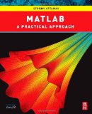
I haven’t had this book as long as I’ve had the Higham book and I haven’t even completely finished it yet. I am, however, very impressed with it (as an aside, it’s also the first technical book I ever bought using the iPad and Android Kindle apps).
One of the key things that I like most about this one is that the text is liberally sprinkled with ‘Quick Questions’ that give you a little scenario and ask you how you’d deal with it in MATLAB. This is quickly followed by a model answer that explains the concepts. These help break up the text, make you stop and think and ultimately lead to you thinking in a more MATLABy way. There is also a good amount of exercises at the end of each chapter (no model solutions provided though).
The book is split into two main parts with the first half concentrating on MATLAB fundamentals such as matrices, vectorization, strings, functions etc while the second half covers mathematical applications such as statistics, curve fitting and numerical integration. So, it’ll take you from being a complete novice to someone who knows their way around a reasonable portion of the system.
Since I first bought this book using the Kindle app on my iPad I thought I’d quickly mention how that worked out for me. In short, I hated the Kindle presentation so much that I went out and bought the physical version of the book as well. The paper version is beautifully formatted and presented whereas the Kindle version is just awful. It’s hard to navigate, looks awful and basically makes one wish that they had just given you a pdf file instead!
MATLAB has a command called reshape that,obviously enough, allows you to reshape a matrix.
mat=rand(4)
mat =
    0.1576    0.8003    0.7922    0.8491
    0.9706    0.1419    0.9595    0.9340
    0.9572    0.4218    0.6557    0.6787
    0.4854    0.9157    0.0357    0.7577

>> reshape(mat,[2,8])
ans =
    0.1576    0.9572    0.8003    0.4218    0.7922    0.6557    0.8491    0.6787
    0.9706    0.4854    0.1419    0.9157    0.9595    0.0357    0.9340    0.7577
Obviously, the number of rows and columns both have to be positive. A negative number of rows and columns makes no sense at all. On MATLAB 2010a:
>> reshape(mat,[-2,-8])
??? Error using ==> reshape
Size vector elements should be nonnegative.
So far so boring. However, I found an old copy of MATLAB on my system (version 6.5.1) which gives much more interesting error messages
>> reshape(mat,[-2,-8])
??? Error using ==> reshape
Don't do this again!.
Obviously, I ignore the warning
>> reshape(mat,[-2,-8])
??? Error using ==> reshape
Cleve says you should be doing something more useful.
Nope, I’ve got nothing better to do
??? Error using ==> reshape
Seriously, size arguments cannot be negative.
I don’t know about you but I prefer the old error messages myself. MATLAB hasn’t completely lost its sense of humour, however, try evaluating the following for example
spy
Not long after publishing my article, A faster version of MATLAB’s fsolve using the NAG Toolbox for MATLAB, I was contacted by Biao Guo of Quantitative Finance Collector who asked me what I could do with the following piece of code.
function MarkowitzWeight = fsolve_markowitz_MATLAB()

RandStream.setDefaultStream (RandStream('mt19937ar','seed',1));
% simulate 500 stocks return
SimR = randn(1000,500);
r = mean(SimR); % use mean return as expected return
targetR = 0.02;
rCOV = cov(SimR); % covariance matrix
NumAsset = length(r);

options=optimset('Display','off');
startX = [1/NumAsset*ones(1, NumAsset), 1, 1];
x = fsolve(@fsolve_markowitz,startX,options, r, targetR, rCOV);
MarkowitzWeight = x(1:NumAsset);
end

function F = fsolve_markowitz(x, r, targetR, rCOV)
NumAsset = length(r);
F = zeros(1,NumAsset+2);
weight = x(1:NumAsset); % for asset weights
lambda = x(NumAsset+1);
mu = x(NumAsset+2);
for i = 1:NumAsset
    F(i) = weight(i)*sum(rCOV(i,:))-lambda*r(i)-mu;
end
F(NumAsset+1) = sum(weight.*r)-targetR;
F(NumAsset+2) = sum(weight)-1;
end
This is an example from financial mathematics and Biao explains it in more detail in a post over at his blog, mathfinance.cn. Now, it isn’t particularly computationally challenging since it only takes 6.5 seconds to run on my 2Ghz dual core laptop. It is, however, significantly more challenging than the toy problem I discussed in my original fsolve post. So, let’s see how much we can optimise it using NAG and any other techniques that come to mind.
Before going on, I’d just like to point out that we intentionally set the seed of the random number generator with
RandStream.setDefaultStream (RandStream('mt19937ar','seed',1));
to ensure we are always operating with the same data set. This is purely for benchmarking purposes.
Optimisation trick 1 – replacing fsolve with NAG’s c05nb
The first thing I had to do to Biao’s code in order to apply the NAG toolbox was to split it into two files. We have the main program, fsolve_markowitz_NAG.m
function MarkowitzWeight = fsolve_markowitz_NAG()
global r targetR rCOV;
%seed random generator to ensure same results every time for benchmark purposes
RandStream.setDefaultStream (RandStream('mt19937ar','seed',1));

% simulate 500 stocks return
SimR = randn(1000,500);
r = mean(SimR)'; % use mean return as expected return
targetR = 0.02;
rCOV = cov(SimR); % covariance matrix
NumAsset = length(r);

startX = [1/NumAsset*ones(1,NumAsset), 1, 1];
tic
x = c05nb('fsolve_obj_NAG',startX);
toc
MarkowitzWeight = x(1:NumAsset);
end
and the objective function, fsolve_obj_NAG.m
function [F,iflag] = fsolve_obj_NAG(n,x,iflag)
global r targetR rCOV;
NumAsset = length(r);
F = zeros(1,NumAsset+2);
weight = x(1:NumAsset); % for asset weights
lambda = x(NumAsset+1);
mu = x(NumAsset+2);
for i = 1:NumAsset
    F(i) = weight(i)*sum(rCOV(i,:))-lambda*r(i)-mu;
end
F(NumAsset+1) = sum(weight.*r)-targetR;
F(NumAsset+2) = sum(weight)-1;
end
I had to put the objective function into its own .m file because because the NAG toolbox currently doesn’t accept function handles (This may change in a future release I am reliably told). This is a pain but not a show stopper.
Note also that the function header for the NAG version of the objective function is different from the pure MATLAB version as
per my original article.
Transposition problems
The next thing to notice is that I have done the following in the main program, fsolve_markowitz_NAG.m
r = mean(SimR)';
compared to the original
r = mean(SimR);
This is because the NAG routine, c05nb, does something rather bizarre. I discovered that if you pass a 1xN matrix to NAGs c05nb then it gets transposed in the objective function to Nx1. Since Biao relies on this being 1xN when he does
F(NumAsset+1) = sum(weight.*r)-targetR;
we get an error unless you take the transpose of r in the main program. I consider this to be a bug in the NAG Toolbox and it is currently with NAG technical support.
Global variables
Sadly, there is no easy way to pass extra variables to the objective function when using NAG’s c05nb. In MATLAB Biao could do this
x = fsolve(@fsolve_markowitz,startX,options, r, targetR, rCOV);
No such luck with c05nb. The only way to get around it is to use global variables (Well, a small lie, there is another way, you can use reverse communication in a different NAG function, c05nd, but that’s a bit more complicated and I’ll leave it for another time I think)
So, It’s pretty clear that the NAG function isn’t as easy to use as MATLAB’s fsolve function but is it any faster? The following is typical.
>> tic;fsolve_markowitz_NAG;toc
Elapsed time is 2.324291 seconds.
So, we have sped up our overall computation time by a factor of 3. Not bad, but nowhere near the 18 times speed-up that I demonstrated in my original post.
Optimisation trick 2 – Don’t sum so much
In his recent blog post, Biao challenged me to make his code almost 20 times faster and after applying my NAG Toolbox trick I had ‘only’ managed to make it 3 times faster. So, in order to see what else I might be able to do for him I ran his code through the MATLAB profiler and discovered that it spent the vast majority of its time in the following section of the objective function
for i = 1:NumAsset
    F(i) = weight(i)*sum(rCOV(i,:))-lambda*r(i)-mu;
end
It seemed to me that the original code was calculating the sum of rCOV too many times. On a small number of assets (50 say) you’ll probably not notice it but with 500 assets, as we have here, it’s very wasteful.
So, I changed the above to
for i = 1:NumAsset
    F(i) = weight(i)*sumrCOV(i)-lambda*r(i)-mu;
end
So,instead of rCOV, the objective function needs to be passed the following in the main program
sumrCOV=sum(rCOV)
We do this summation once and once only and make a big time saving. This is done in the files fsolve_markowitz_NAGnew.m and fsolve_obj_NAGnew.m
With this optimisation, along with using NAG’s c05nb we now get the calculation time down to
>> tic;fsolve_markowitz_NAGnew;toc
Elapsed time is 0.203243 seconds.
Compared to the 6.5 seconds of the original code, this represents a speed-up of over 32 times. More than enough to satisfy Biao’s challenge.
Checking the answers
Let’s make sure that the results agree with each other. I don’t expect them to be exactly equal due to round off errors etc but they should be extremely close. I check that the difference between each result is less than 1e-7:
original_results = fsolve_markowitz_MATLAB;
nagver1_results = fsolve_markowitz_NAGnew;
>> all(abs(original_results - nagver1_results)<1e8)
ans =
     1
That’ll do for me!
Summary
The current iteration of the NAG Toolbox for MATLAB (Mark 22) may not be as easy to use as native MATLAB toolbox functions (for this example at least) but it can often provide useful speed-ups and in this example, NAG gave us a factor of 3 improvement compared to using fsolve.
For this particular example, however, the more impressive speed-up came from pushing the code through the MATLAB profiler, identifying the hotspot and then doing something about it. There are almost certainly more optimisations to make but with the code running at less than a quarter of a second on my modest little laptop I think we will leave it there for now.
Part of my job at the University of Manchester is to help researchers improve their code in systems such as Mathematica, MATLAB, NAG and so on. One of the most common questions I get asked is ‘Can you make this go any faster please?’ and it always makes my day if I manage to do something significant such as a speed up of a factor of 10 or more. The users, however, are often happy with a lot less and I once got bought a bottle of (rather good) wine for a mere 25% speed-up (Note: Gifts of wine aren’t mandatory)
I employ numerous tricks to get these speed-ups including applying vectorisation, using mex files, modifying the algorithm to something more efficient,picking the brains of colleagues and so on. Over the last year or so, I have managed to help several researchers get significant speed-ups in their MATLAB programs by doing one simple thing – swapping the fsolve function for an equivalent from the NAG Toolbox for MATLAB.
The fsolve function is part of MATLAB’s optimisation toolbox and, according to the documentation, it does the following:
“fsolve Solves a system of nonlinear equation of the form F(X) = 0 where F and X may be vectors or matrices.”
The NAG Toolbox for MATLAB contains a total of 6 different routines that can perform similar calculations to fsolve. These 6 routines are split into 2 sets of 3 as follows
For when you have function values only:
c05nb – Solution of system of nonlinear equations using function values only (easy-to-use)
c05nc – Solution of system of nonlinear equations using function values only (comprehensive)
c05nd – Solution of system of nonlinear equations using function values only (reverse communication)
For when you have both function values and first derivatives
c05pb – Solution of system of nonlinear equations using first derivatives (easy-to-use)
c05pc – Solution of system of nonlinear equations using first derivatives (comprehensive)
c05pd – Solution of system of nonlinear equations using first derivatives (reverse communication)
So, the NAG routine you choose depends on whether or not you can supply first derivatives and exactly which options you’d like to exercise. For many problems it will come down to a choice between the two ‘easy to use’ routines – c05nb and c05pb (at least, they are the ones I’ve used most of the time)
Let’s look at a simple example. You’d like to find a root of the following system of non-linear equations.
F(1)=exp(-x(1)) + sinh(2*x(2)) + tanh(2*x(3)) – 5.01;
F(2)=exp(2*x(1)) + sinh(-x(2) ) + tanh(2*x(3) ) – 5.85;
F(3)=exp(2*x(1)) + sinh(2*x(2) ) + tanh(-x(3) ) – 8.88;
i.e. you want to find a vector X containing three values for which F(X)=0.
To solve this using MATLAB and the optimisation toolbox you could proceed as follows, first create a .m file called fsolve_obj_MATLAB.m (henceforth referred to as the objective function) that contains the following
function  F=fsolve_obj_MATLAB(x)
F=zeros(1,3);
F(1)=exp(-x(1))  + sinh(2*x(2)) + tanh(2*x(3)) - 5.01;
F(2)=exp(2*x(1)) +  sinh(-x(2) ) + tanh(2*x(3) ) - 5.85;
F(3)=exp(2*x(1)) +  sinh(2*x(2) ) + tanh(-x(3) ) - 8.88;
end
Now type the following at the MATLAB command prompt to actually solve the problem:
options=optimset('Display','off'); %Prevents fsolve from  displaying too much information
startX=[0 0 0]; %Our  starting guess for the solution vector
X=fsolve(@fsolve_obj_MATLAB,startX,options)
MATLAB finds the following solution (Note that it’s only found one of the solutions, not all of them, which is typical of the type of algorithm used in fsolve)
X =
0.9001     1.0002    1.0945
Since we are not supplying the derivatives of our objective function and we are not using any special options, it turns out to be very easy to switch from using the optimisation toolbox to the NAG toolbox for this particular problem by making use of the routine c05nb.
First, we need to change the header of our objective function’s .m file from
function F=fsolve_obj_MATLAB(x)
to
function [F,iflag]=fsolve_obj_NAG(n,x,iflag)
so our new .m file, fsolve_obj_NAG.m, will contain the following
function  [F,iflag]=fsolve_obj_NAG(n,x,iflag)
F=zeros(1,3);
F(1)=exp(-x(1)) + sinh(2*x(2)) + tanh(2*x(3)) - 5.01;
F(2)=exp(2*x(1)) + sinh(-x(2) ) + tanh(2*x(3) ) - 5.85;
F(3)=exp(2*x(1)) + sinh(2*x(2) ) + tanh(-x(3) ) - 8.88;
end
Note that the ONLY change we made to the objective function was the very first line. The NAG routine c05nb expects to see some extra arguments in the objective function (iflag and n in this example) and it expects to see them in a very particular order but we are not obliged to use them. Using this modified objective function we can proceed as follows.
startX=[0 0 0]; %Our starting guess
X=c05nb('fsolve_obj_NAG',startX)
NAG gives the same result as the optimisation toolbox:
X =
0.9001    1.0002    1.0945
Let’s look at timings. I performed the calculations above on an 800Mhz laptop running Ubuntu Linux 10.04, MATLAB 2009 and Mark 22 of the NAG toolbox and got the following timings (averaged over 10 runs):
Optimisation toolbox: 0.0414 seconds
NAG toolbox: 0.0021 seconds
So, for this particular problem NAG was faster than MATLAB by a factor of 19.7 times on my machine.
That’s all well and good, but this is a simple problem. Does this scale to more realistic problems I hear you ask? Well, the answer is ‘yes’. I’ve used this technique several times now on production code and it almost always results in some kind of speed-up. Not always 19.7 times faster, I’ll grant you, but usually enough to make the modifications worthwhile.
I can’t actually post any of the more complicated examples here because the code in question belongs to other people but I was recently sent a piece of code from a researcher that made heavy use of fsolve and a typical run took 18.19 seconds (that’s for everything, not just the fsolve bit). Simply by swapping a couple of lines of code to make it use the NAG toolbox rather than the optimisation toolbox I reduced the runtime to 1.08 seconds – a speed-up of almost 17 times.
Sadly, this technique doesn’t always result in a speed-up and I’m working on figuring out exactly when the benefits disappear. I guess that the main reason for NAG’s good performance is that it uses highly optimised, compiled Fortran code compared to MATLAB’s interpreted .m code. One case where NAG didn’t help was for a massively complicated objective function and the majority of the run-time of the code was spent evaluating this function. In this situation, NAG and MATLAB came out roughly neck and neck.
In the meantime, if you have some code that you’d like me to try it on then drop me a line.
If you enjoyed this post then you may also like:
A very welcome change in MATLAB 2010b is the merging of the splines and curve-fitting toolboxes to form one super-toolbox that does both splines AND curve-fitting in a product that’s simply called The Curve Fitting Toolbox. The separate curve-fitting and splines toolboxes were always a bugbear for me and many of my equivalents in other UK universities so now we have one less thing to moan about. Thanks to the HUGE number of MATLAB toolboxes, however, we’ll still have plenty of things to moan about at our quarterly academic maths and stats meetings.
I took a trawl through some of Mathworks standard toolboxes to see what other toolboxes I thought should be merged together or done away with completely. Here are a couple of pleas to The Mathworks that would make MY life (and the lives of the community I support) a whole lot easier.
The Parallel Toolbox for MATLAB
My laptop has a dual core processor so, unless I am lucky enough to be using functions that are implicitly parallel, MATLAB will only make use of half of my available processing power. It gets worse when I get into work since it will only use a quarter of the power of my quad-core desktop and as for those lucky fellows who have just bought themselves dual hex-core MONSTERS (12 cores total)….well, MATLAB won’t exactly be using them to their full capacity will it? Less than 10% in fact, unless they shell out extra for the parallel computing toolbox (PCT).
The vast majority of computers sold today have more than one processing core and yet the vast majority of MATLAB installations out there only use one of them (unless you use these functions). MATLAB’s competitors such as Mathematica, Maple and Labview all have explicit multi-core support built in as standard. Maybe it’s time that MATLAB did that too!
What I’d like Mathworks to do:Merge the Parallel Computing Toolbox with core MATLAB.
Optimisation and Global Optimisation
You’ve got a function and you want to know when it gets as big or as small as it can be so you turn to optimisation routines. MATLAB has some basic optimisation functions built into its core (fminsearch for example) but many people find that they need the extra power and versatility offered by the functions in either the optimisation toolbox or the global optimisation toolbox.
People who have never used optimisation routines before sometimes ask me what the difference between these toolboxes is. When I was first faced with this question I discussed the different classes of algorithms involved and used phrases like ‘genetic algorithms’, ‘multistart’, ‘simulated annealing’, ‘global and local minima’ and so on. These days I start off somewhat more simply:
Me: “The optimisation toolbox finds A minimum near to your starting guess. It may or may not be THE minimum of your function. The global optimisation toolbox, on the other hand, attempts to find THE minimum.”
User: “Well, I want THE minimum obviously. So, I guess I’ll take the global optimisation toolbox please.”
Me: THE minimum costs more money than just A minimum. Twice as much in fact, since you need to buy the standard optimisation toolbox AND the global optimisation toolbox if you want THE minimum.
User: <Deep in thought while they consider how far their grant is going to stretch>
Me: The standard optimisation toolbox won’t cost you anything here since we have a set of licenses for it on our network license server.
User: OK OK. I’ll make do with that. I suppose I could just make LOTS of starting guesses and run the standard optimisation toolbox routines in parallel on my 12-core monster? Then I can take the best result and there will be a better chance that it will be THE minimum, right?
Me: That’ll need the Parallel computing toolbox…which costs extra!
What I’d like Mathworks to do: Merge the standard and global optimisation toolboxes.
So, that’s a couple of things that I would like. Do you agree with them? Are there other toolbox merges you’d like to see? Comments welcome.