
Archive for the ‘matlab’ Category
So, you’re the proud owner of a new license for MATLAB’s parallel computing toolbox (PCT) and you are wondering how to get some bang for your buck as quickly as possible. Sure, you are going to learn about constructs such as parfor and spmd but that takes time and effort. Wouldn’t it be nice if you could speed up some of your MATLAB code simply by saying ‘Turn parallelisation on’?
It turns out that The Mathworks have been adding support for their parallel computing toolbox all over the place and all you have to do is switch it on (Assuming that you actually have the parallel computing toolbox of course). For example say you had the following call to fmincon (part of the optimisation toolbox) in your code
[x, fval] = fmincon(@objfun, x0, [], [], [], [], [], [], @confun,opts)
To turn on parallelisation across 2 cores just do
matlabpool 2;
opts = optimset('fmincon');
opts = optimset('UseParallel','always');
[x, fval] = fmincon(@objfun, x0, [], [], [], [], [], [], @confun,opts);
That wasn’t so hard was it? The speedup (if any) completely depends upon your particular optimization problem.
Why isn’t parallelisation turned on by default?
The next question that might occur to you is ‘Why doesn’t The Mathworks just turn parallelisation on by default?’ After all, although the above modification is straightforward, it does require you to know that this particular function supports parallel execution via the PCT. If you didn’t think to check then your code would be doomed to serial execution forever.
The simple answer to this question is ‘Sometimes the parallel version is slower‘. Take this serial code for example.
objfun = @(x)exp(x(1))*(4*x(1)^2+2*x(2)^2+4*x(1)*x(2)+2*x(2)+1);
confun = @(x) deal( [1.5+x(1)*x(2)-x(1)-x(2); -x(1)*x(2)-10], [] );
tic;
[x, fval] = fmincon(objfun, x0, [], [], [], [], [], [], confun);
toc
On the machine I am currently sat at (quad core running MATLAB 2011a on Linux) this typically takes around 0.032 seconds to solve. With a problem that trivial my gut feeling is that we are not going to get much out of switching to parallel mode.
objfun = @(x)exp(x(1))*(4*x(1)^2+2*x(2)^2+4*x(1)*x(2)+2*x(2)+1);
confun = @(x) deal( [1.5+x(1)*x(2)-x(1)-x(2); -x(1)*x(2)-10],[] );

%only do this next line once.  It opens two MATLAB workers
matlabpool 2;

opts = optimset('fmincon');
opts = optimset('UseParallel','always');

tic;
[x, fval] = fmincon(objfun, x0, [], [], [], [], [], [], confun,opts);
toc
Sure enough, this increases execution time dramatically to an average of 0.23 seconds on my machine. There is always a computational overhead that needs paying when you go parallel and if your problem is too trivial then this overhead costs more than the calculation itself.
So which functions support the Parallel Computing Toolbox?
I wanted a web-page that listed all functions that gain benefit from the Parallel Computing Toolbox but couldn’t find one. I found some documentation on specific toolboxes such as Parallel Statistics but nothing that covered all of MATLAB in one place. Here is my attempt at producing such a document. Feel free to contact me if I have missed anything out.
This covers MATLAB 2011b and is almost certainly incomplete. I’ve only covered toolboxes that I have access to and so some are missing. Please contact me if you have any extra information.
Bioinformatics Toolbox
Global Optimisation
- Various solvers use the PCT. See this part of the MATLAB documentation for details.
Image Processing
- blockproc
- Note that many Image Processing functions run in parallel even without the parallel computing toolbox. See my article Which MATLAB functions are Multicore Aware?
Optimisation Toolbox
Simulink
- Running parallel simulations
- You can increase the speed of diagram updates for models containing large model reference hierarchies by building referenced models that are configured in Accelerator mode in parallel whenever conditions allow. This is covered in the documentation.
Statistics Toolbox
- bootstrp
- bootci
- cordexch
- candexch
- crossval
- dcovary
- daugment
- growTrees
- jackknife
- lasso
- nnmf
- plsregress
- rowexch
- sequentialfs
- TreeBagger
Other articles about parallel computing in MATLAB from WalkingRandomly
- Which MATLAB functions are multicore aware? There are a ton of functions in MATLAB that take advantage of parallel processors automatically. No Parallel Computing Toolbox necessary.
- Parallel MATLAB with OpenMP mex files Want to parallelize your own functions without purchasing the PCT? Not afraid to get your hands dirty with C? Perhaps this option is for you.
- MATLAB GPU/CUDA Experiences and tutorials on my laptop – A series of articles where I look a GPU computing with CUDA on MATLAB
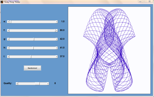
Matt Tearle has produced a MATLAB version of my Interactive Slinky Thing which, in turn, was originally inspired by a post by Sol over at Playing with Mathematica. Matt adatped the code from some earlier work he did and you can click on the image below to get it. Thanks Matt!
This is part 2 of an ongoing series of articles about MATLAB programming for GPUs using the Parallel Computing Toolbox. The introduction and index to the series is at https://www.walkingrandomly.com/?p=3730. All timings are performed on my laptop (hardware detailed at the end of this article) unless otherwise indicated.
Last time
In the previous article we saw that it is very easy to run MATLAB code on suitable GPUs using the parallel computing toolbox. We also saw that the GPU has its own area of memory that is completely separate from main memory. So, if you have a program that runs in main memory on the CPU and you want to accelerate part of it using the GPU then you’ll need to explicitly transfer data to the GPU and this takes time. If your GPU calculation is particularly simple then the transfer times can completely swamp your performance gains and you may as well not bother.
So, the moral of the story is either ‘Keep data transfers between GPU and host down to a minimum‘ or ‘If you are going to transfer a load of data to or from the GPU then make sure you’ve got a ton of work for the GPU to do.‘ Today, I’m going to consider the latter case.
A more complicated elementwise function – CPU version
Last time we looked at a very simple elementwise calculation– taking the sine of a large array of numbers. This time we are going to increase the complexity ever so slightly. Consider trig_series.m which is defined as follows
function out = myseries(t)
  out = 2*sin(t)-sin(2*t)+2/3*sin(3*t)-1/2*sin(4*t)+2/5*sin(5*t)-1/3*sin(6*t)+2/7*sin(7*t);
end
Let’s generate 75 million random numbers and see how long it takes to apply this function to all of them.
cpu_x = rand(1,75*1e6)*10*pi;
tic;myseries(cpu_x);toc
I did the above calculation 20 times using a for loop and took the median of the results to get 4.89 seconds1. Note that this calculation is fully parallelised…all 4 cores of my i7 CPU were working on the problem simultaneously (Many built in MATLAB functions are parallelised these days by the way…No extra toolbox necessary).
GPU version 1 (Or ‘How not to do it’)
One way of performing this calculation on the GPU would be to proceed as follows
cpu_x =rand(1,75*1e6)*10*pi;
tic
%Transfer data to GPU
gpu_x = gpuArray(cpu_x);
%Do calculation using GPU
gpu_y = myseries(gpu_x);
%Transfer results back to main memory
cpu_y = gather(gpu_y)
toc
The mean time of the above calculation on my laptop’s GPU is 3.27 seconds, faster than the CPU version but not by much. If you don’t include data transfer times in the calculation then you end up with 2.74 seconds which isn’t even a factor of 2 speed-up compared to the CPU.
GPU version 2 (arrayfun to the rescue)
We can get better performance out of the GPU simply by changing the line that does the calculation from
gpu_y = myseries(gpu_x);
to a version that uses MATLAB’s arrayfun command.
gpu_y = arrayfun(@myseries,gpu_x);
So, the full version of the code is now
cpu_x =rand(1,75*1e6)*10*pi;
tic
%Transfer data to GPU
gpu_x = gpuArray(cpu_x);
%Do calculation using GPU via arrayfun
gpu_y = arrayfun(@myseries,gpu_x);
%Transfer results back to main memory
cpu_y = gather(gpu_y)
toc
This improves the timings quite a bit. If we don’t include data transfer times then the arrayfun version completes in 1.42 seconds down from 2.74 seconds for the original GPU code. Including data transfer, the arrayfun version complete in 1.94 seconds compared to for the 3.27 seconds for the original.
Using arrayfun for the GPU is definitely the way to go! Giving the GPU every disadvantage I can think of (double precision, including transfer times, comparing against multi-thread CPU code etc) we still get a speed-up of just over 2.5 times on my laptop’s hardware. Pretty useful for hardware that was designed for energy-efficient gaming!
Note: Something that I learned while writing this post is that the first call to arrayfun will be slower than all of the rest. This is because arrayfun compiles the MATLAB function you pass it down to PTX and this can take a while (seconds). Subsequent calls will be much faster since arrayfun will use the compiled results. The compiled PTX functions are not saved between MATLAB sessions.
arrayfun – Good for your memory too!
Using the arrayfun function is not only good for performance, it’s also good for memory management. Imagine if I had 100 million elements to operate on instead of only 75 million. On my 3Gb GPU, the following code fails:
cpu_x = rand(1,100*1e6)*10*pi;
gpu_x = gpuArray(cpu_x);
gpu_y = myseries(gpu_x);
??? Error using ==> GPUArray.mtimes at 27
Out of memory on device. You requested: 762.94Mb, device has 724.21Mb free.

Error in ==> myseries at 3
        out =
        2*sin(t)-sin(2*t)+2/3*sin(3*t)-1/2*sin(4*t)+2/5*sin(5*t)-1/3*sin(6*t)+2/7*sin(7*t);
If we use arrayfun, however, then we are in clover. The following executes without complaint.
cpu_x = rand(1,100*1e6)*10*pi;
gpu_x = gpuArray(cpu_x);
gpu_y = arrayfun(@myseries,gpu_x);
Some Graphs
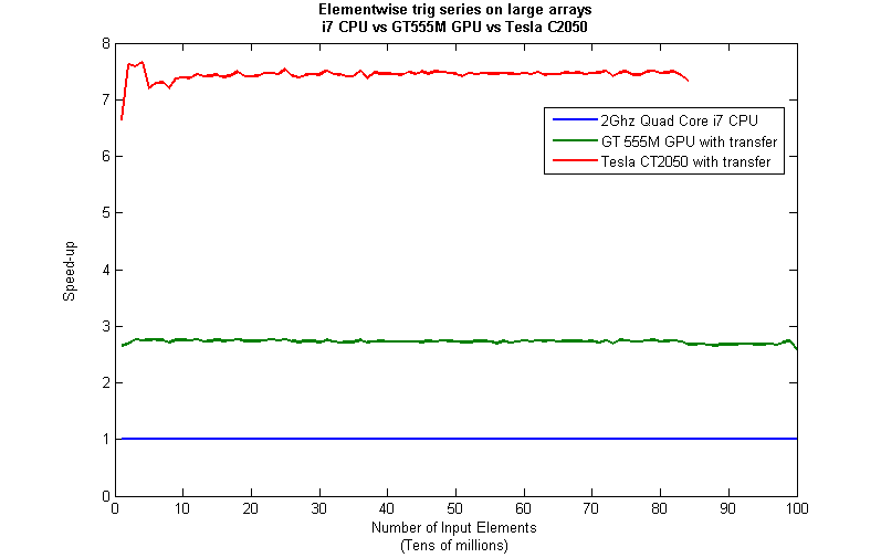
Just like last time, I ran this calculation on a range of input arrays from 1 million to 100 million elements on both my laptop’s GT 555M GPU and a Tesla C2050 I have access to. Unfortunately, the C2050 is running MATLAB 2010b rather than 2011a so it’s not as fair a test as I’d like. I could only get up to 84 million elements on the Tesla before it exited due to memory issues. I’m not sure if this is down to the hardware itself or the fact that it was running an older version of MATLAB.

Next, I looked at the actual speed-up shown by the GPUs compared to my laptop’s i7 CPU. Again, this includes data transfer times, is in full double precision and the CPU version was multi-threaded (No dodgy ‘GPUs are awesome’ techniques used here). No matter what array size is used I get almost a factor of 3 speed-up using the laptop GPU and more than a factor of 7 speed-up when using the Tesla. Not too shabby considering that the programming effort to achieve this speed-up was minimal.
Conclusions
- It is VERY easy to modify simple, element-wise functions to take advantage of the GPU in MATLAB using the Parallel Computing Toolbox.
- arrayfun is the most efficient way of dealing with such functions.
- My laptop’s GPU demonstrated almost a 3 times speed-up compared to its CPU.
Hardware / Software used for the majority of this article
- Laptop model: Dell XPS L702X
- CPU: Intel Core i7-2630QM @2Ghz software overclockable to 2.9Ghz. 4 physical cores but total 8 virtual cores due to Hyperthreading.
- GPU: GeForce GT 555M with 144 CUDA Cores. Graphics clock: 590Mhz. Processor Clock:1180 Mhz. 3072 Mb DDR3 Memeory
- RAM: 8 Gb
- OS: Windows 7 Home Premium 64 bit. I’m not using Linux because of the lack of official support for Optimus.
- MATLAB: 2011a with the parallel computing toolbox
Code and sample timings (Will grow over time)
You need myseries.m and trigseries_test.m and the Parallel Computing Toolbox. These are the times given by the following function call for various systems (transfer included and using arrayfun).
[cpu,~,~,~,gpu] = trigseries_test(10,50*1e6,'mean')
GPUs
- Tesla C2050, Linux, 2010b – 0.4751 seconds
- NVIDIA GT 555M – 144 CUDA Cores, 3Gb RAM, Windows 7, 2011a – 1.2986 seconds
CPUs
- Intel Core i7-2630QM, Windows 7, 2011a (My laptop’s CPU) – 3.33 seconds
- Intel Core 2 Quad Q9650 @ 3.00GHz, Linux, 2011a – 3.9452 seconds
Footnotes
1 – This is the method used in all subsequent timings and is similar to that used by the File Exchange function, timeit (timeit takes a median, I took a mean). If you prefer to use timeit then the function call would be timeit(@()myseries(cpu_x)). I stick to tic and toc in the article because it makes it clear exactly where timing starts and stops using syntax well known to most MATLABers.
Thanks to various people at The Mathworks for some useful discussions, advice and tutorials while creating this series of articles.
This is part 1 of an ongoing series of articles about MATLAB programming for GPUs using the Parallel Computing Toolbox. The introduction and index to the series is at https://www.walkingrandomly.com/?p=3730.
Have you ever needed to take the sine of 100 million random numbers? Me either, but such an operation gives us an excuse to look at the basic concepts of GPU computing with MATLAB and get an idea of the timings we can expect for simple elementwise calculations.
Taking the sine of 100 million numbers on the CPU
Let’s forget about GPUs for a second and look at how this would be done on the CPU using MATLAB. First, I create 100 million random numbers over a range from 0 to 10*pi and store them in the variable cpu_x;
cpu_x = rand(1,100000000)*10*pi;
Now I take the sine of all 100 million elements of cpu_x using a single command.
cpu_y = sin(cpu_x)
I have to confess that I find the above command very cool. Not only are we looping over a massive array using just a single line of code but MATLAB will also be performing the operation in parallel. So, if you have a multicore machine (and pretty much everyone does these days) then the above command will make good use of many of those cores. Furthermore, this kind of parallelisation is built into the core of MATLAB….no parallel computing toolbox necessary. As an aside, if you’d like to see a list of functions that automatically run in parallel on the CPU then check out my blog post on the issue.
So, how quickly does my 4 core laptop get through this 100 million element array? We can find out using the MATLAB functions tic and toc. I ran it three times on my laptop and got the following
>> tic;cpu_y = sin(cpu_x);toc
Elapsed time is 0.833626 seconds.
>> tic;cpu_y = sin(cpu_x);toc
Elapsed time is 0.899769 seconds.
>> tic;cpu_y = sin(cpu_x);toc
Elapsed time is 0.916969 seconds.
So the first thing you’ll notice is that the timings vary and I’m not going to go into the reasons why here. What I am going to say is that because of this variation it makes sense to time the calculation a number of times (20 say) and take an average. Let’s do that
sintimes=zeros(1,20);
for i=1:20;tic;cpu_y = sin(cpu_x);sintimes(i)=toc;end
average_time = sum(sintimes)/20

average_time =
    0.8011
So, on average, it takes my quad core laptop just over 0.8 seconds to take the sine of 100 million elements using the CPU. A couple of points:
- I note that this time is smaller than any of the three test times I did before running the loop and I’m not really sure why. I’m guessing that it takes my CPU a short while to decide that it’s got a lot of work to do and ramp up to full speed but further insights are welcomed.
- While staring at the CPU monitor I noticed that the above calculation never used more than 50% of the available virtual cores. It’s using all 4 of my physical CPU cores but perhaps if it took advantage of hyperthreading I’d get even better performance? Changing OMP_NUM_THREADS to 8 before launching MATLAB did nothing to change this.
Taking the sine of 100 million numbers on the GPU
Just like before, we start off by using the CPU to generate the 100 million random numbers1
cpu_x = rand(1,100000000)*10*pi;
The first thing you need to know about GPUs is that they have their own memory that is completely separate from main memory. So, the GPU doesn’t know anything about the array created above. Before our GPU can get to work on our data we have to transfer it from main memory to GPU memory and we acheive this using the gpuArray command.
gpu_x = gpuArray(cpu_x); %this moves our data to the GPU
Once the GPU can see all our data we can apply the sine function to it very easily.
gpu_y = sin(gpu_x)
Finally, we transfer the results back to main memory.
cpu_y = gather(gpu_y)
If, like many of the GPU articles you see in the literature, you don’t want to include transfer times between GPU and host then you time the calculation like this:
tic
gpu_y = sin(gpu_x);
toc
Just like the CPU version, I repeated this calculation several times and took an average. The result was 0.3008 seconds giving a speedup of 2.75 times compared to the CPU version.
If, however, you include the time taken to transfer the input data to the GPU and the results back to the CPU then you need to time as follows
tic
gpu_x = gpuArray(cpu_x);
gpu_y = sin(gpu_x);
cpu_y = gather(gpu_y)
toc
On my system this takes 1.0159 seconds on average– longer than it takes to simply do the whole thing on the CPU. So, for this particular calculation, transfer times between host and GPU swamp the benefits gained by all of those CUDA cores.
Benchmark code
I took the ideas above and wrote a simple benchmark program called sine_test. The way you call it is as follows
[cpu,gpu_notransfer,gpu_withtransfer] = sin_test(numrepeats,num_elements]
For example, if you wanted to run the benchmarks 20 times on a 1 million element array and return the average times then you just do
>> [cpu,gpu_notransfer,gpu_withtransfer] = sine_test(20,1e6)
cpu =
    0.0085
gpu_notransfer =
    0.0022
gpu_withtransfer =
    0.0116
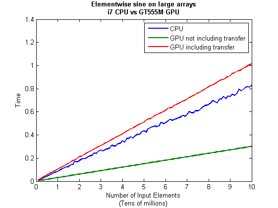
I then ran this on my laptop for array sizes ranging from 1 million to 100 million and used the results to plot the graph below.
But I wanna write a ‘GPUs are awesome’ paper
So far in this little story things are not looking so hot for the GPU and yet all of the ‘GPUs are awesome’ papers you’ve ever read seem to disagree with me entirely. What on earth is going on? Well, lets take the advice given by csgillespie.wordpress.com and turn it on its head. How do we get awesome speedup figures from the above benchmarks to help us pump out a ‘GPUs are awesome paper’?
0. Don’t consider transfer times between CPU and GPU.
We’ve already seen that this can ruin performance so let’s not do it shall we? As long as we explicitly say that we are not including transfer times then we are covered.
1. Use a singlethreaded CPU.
Many papers in the literature compare the GPU version with a single-threaded CPU version and yet I’ve been using all 4 cores of my processor. Silly me…let’s fix that by running MATLAB in single threaded mode by launching it with the command
matlab -singleCompThread
Now when I run the benchmark for 100 million elements I get the following times
>> [cpu,gpu_no,gpu_with] = sine_test(10,1e8)
cpu =
    2.8875
gpu_no =
    0.3016
gpu_with =
    1.0205
Now we’re talking! I can now claim that my GPU version is over 9 times faster than the CPU version.
2. Use an old CPU.
My laptop has got one of those new-fangled sandy-bridge i7 processors…one of the best classes of CPU you can get for a laptop. If, however, I was doing these tests at work then I guess I’d be using a GPU mounted in my university Desktop machine. Obviously I would compare the GPU version of my program with the CPU in the Desktop….an Intel Core 2 Quad Q9650. Heck its running at 3Ghz which is more Ghz than my laptop so to the casual observer (or a phb) it would look like I was using a more beefed up processor in order to make my comparison fairer.
So, I ran the CPU benchmark on that (in singleCompThread mode obviously) and got 4.009 seconds…noticeably slower than my laptop. Awesome…I am definitely going to use that figure!
I know what you’re thinking…Mike’s being a fool for the sake of it but csgillespie.wordpress.com puts it like this ‘Since a GPU has (usually) been bought specifically for the purpose of the article, the CPU can be a few years older.’ So, some of those ‘GPU are awesome’ articles will be accidentally misleading us in exactly this manner.
3. Work in single precision.
Yeah I know that you like working with double precision arithmetic but that slows GPUs down. So, let’s switch to single precision. Just argue in your paper that single precision is OK for this particular calculation and we’ll be set. To change the benchmarking code all you need to do is change every instance of
rand(1,num_elems)*10*pi;
to
rand(1,num_elems,'single')*10*pi;
Since we are reputable researchers we will, of course, modify both the CPU and GPU versions to work in single precision. Timings are below
- Desktop at work (single thread, single precision): 3.49 seconds
- Laptop GPU (single precision, not including transfer): 0.122 seconds
OK, so switching to single precision made the CPU version a bit faster but it’s more than doubled GPU performance. We can now say that the GPU version is over 28 times faster than the CPU version. Now we have ourselves a bone-fide ‘GPUs are awesome’ paper.
4. Use the best GPU we can find
So far I have been comparing the CPU against the relatively lowly GPU in my laptop. Obviously, however, if I were to do this for real then I’d get a top of the range Tesla. It turns out that I know someone who has a Tesla C2050 and so we ran the single precision benchmark on that. The result was astonishing…0.0295 seconds for 100 million numbers not including transfer times. The double precision performance for the same calculation on the C2050 was 0.0524 seonds.
5. Write the abstract for our ‘GPUs are awesome’ paper
We took an Nvidia Tesla C2050 GPU and mounted it in a machine containing an Intel Quad Core CPU running at 3Ghz. We developed a program that performs element-wise trigonometry on arrays of up to 100 million single precision random numbers using both the CPU and the GPU. The GPU version of our code ran up to 118 times faster than the CPU version. GPUs are awesome!
Results from different CPUs and GPUs. Double precision, multi-threaded
I ran the sine_test benchmark on several different systems for 100 million elements. The CPU was set to be multi-threaded and double precision was used throughout.
sine_test(10,1e8)
GPUs
- Tesla C2050, Linux, 2011a – 0.7487 seconds including transfers, 0.0524 seconds excluding transfers.
- GT 555M – 144 CUDA Cores, 3Gb RAM, Windows 7, 2011a (My laptop’s GPU) -1.0205 seconds including transfers, 0.3016 seconds excluding transfers
CPUs
- Intel Core i7-880 @3.07Ghz, Linux, 2011a – 0.659 seconds
- Intel Core i7-2630QM, Windows 7, 2011a (My laptop’s CPU) – 0.801 seconds
- Intel Core 2 Quad Q9650 @ 3.00GHz, Linux – 0.958 seconds
Conclusions
- MATLAB’s new GPU functions are very easy to use! No need to learn low-level CUDA programming.
- It’s very easy to massage CPU vs GPU numbers to look impressive. Read those ‘GPUs are awesome’ papers with care!
- In real life you have to consider data transfer times between GPU and CPU since these can dominate overall wall clock time with simple calculations such as those considered here. The more work you can do on the GPU, the better.
- My laptop’s GPU is nowhere near as good as I would have liked it to be. Almost 6 times slower than a Tesla C2050 (excluding data transfer) for elementwise double precision calculations. Data transfer times seem to about the same though.
Next time
In the next article in the series I’ll look at an element-wise calculation that really is worth doing on the GPU – even using the wimpy GPU in my laptop – and introduce the MATLAB function arrayfun.
Footnote
1 – MATLAB 2011a can’t create random numbers directly on the GPU. I have no doubt that we’ll be able to do this in future versions of MATLAB which will change the nature of this particular calculation somewhat. Then it will make sense to include the random number generation in the overall benchmark; transfer times to the GPU will be non-existant. In general, however, we’ll still come across plenty of situations where we’ll have a huge array in main memory that needs to be transferred to the GPU for further processing so what we learn here will not be wasted.
Hardware / Software used for the majority of this article
- Laptop model: Dell XPS L702X
- CPU: Intel Core i7-2630QM @2Ghz software overclockable to 2.9Ghz. 4 physical cores but total 8 virtual cores due to Hyperthreading.
- GPU: GeForce GT 555M with 144 CUDA Cores. Graphics clock: 590Mhz. Processor Clock:1180 Mhz. 3072 Mb DDR3 Memeory
- RAM: 8 Gb
- OS: Windows 7 Home Premium 64 bit. I’m not using Linux because of the lack of official support for Optimus.
- MATLAB: 2011a with the parallel computing toolbox
Other GPU articles at Walking Randomly
- GPU Support in Mathematica, Maple, MATLAB and Maple Prime – See the various options available
- Insert new laptop to continue – My first attempt at using the GPU functionality in MATLAB
- NVIDIA lets down Linux laptop users – and how an open source project saves the day
Thanks to various people at The Mathworks for some useful discussions, advice and tutorials while creating this series of articles.
These days it seems that you can’t talk about scientific computing for more than 5 minutes without somone bringing up the topic of Graphics Processing Units (GPUs). Originally designed to make computer games look pretty, GPUs are massively parallel processors that promise to revolutionise the way we compute.
A brief glance at the specification of a typical laptop suggests why GPUs are the new hotness in numerical computing. Take my new one for instance, a Dell XPS L702X, which comes with a Quad-Core Intel i7 Sandybridge processor running at up to 2.9Ghz and an NVidia GT 555M with a whopping 144 CUDA cores. If you went back in time a few years and told a younger version of me that I’d soon own a 148 core laptop then young Mike would be stunned. He’d also be wondering ‘What’s the catch?’
Of course the main catch is that all processor cores are not created equally. Those 144 cores in my GPU are, individually, rather wimpy when compared to the ones in the Intel CPU. It’s the sheer quantity of them that makes the difference. The question at the forefront of my mind when I received my shiny new laptop was ‘Just how much of a difference?’
Now I’ve seen lots of articles that compare CPUs with GPUs and the GPUs always win…..by a lot! Dig down into the meat of these articles, however, and it turns out that things are not as simple as they seem. Roughly speaking, the abstract of some them could be summed up as ‘We took a serial algorithm written by a chimpanzee for an old, outdated CPU and spent 6 months parallelising and fine tuning it for a top of the line GPU. Our GPU version is up to 150 times faster!‘
Well it would be wouldn’t it?! In other news, Lewis Hamilton can drive his F1 supercar around Silverstone faster than my dad can in his clapped out 12 year old van! These articles are so prevalent that csgillespie.wordpress.com recently published an excellent article that summarised everything you should consider when evaluating them. What you do is take the claimed speed-up, apply a set of common sense questions and thus determine a realistic speedup. That factor of 150 can end up more like a factor of 8 once you think about it the right way.
That’s not to say that GPUs aren’t powerful or useful…it’s just that maybe they’ve been hyped up a bit too much!
So anyway, back to my laptop. It doesn’t have a top of the range GPU custom built for scientific computing, instead it has what Notebookcheck.net refers to as a fast middle class graphics card for laptops. It’s got all of the required bits though….144 cores and CUDA compute level 2.1 so surely it can whip the built in CPU even if it’s just by a little bit?
I decided to find out with a few randomly chosen tests. I wasn’t aiming for the kind of rigor that would lead to a peer reviewed journal but I did want to follow some basic rules at least
- I will only choose algorithms that have been optimised and parallelised for both the CPU and the GPU.
- I will release the source code of the tests so that they can be critised and repeated by others.
- I’ll do the whole thing in MATLAB using the new GPU functionality in the parallel computing toolbox. So, to repeat my calculations all you need to do is copy and paste some code. Using MATLAB also ensures that I’m using good quality code for both CPU and GPU.
The articles
This is the introduction to a set of articles about GPU computing on MATLAB using the parallel computing toolbox. Links to the rest of them are below and more will be added in the future.
- Elementwise operations on the GPU #1 – Basic commands using the PCT and how to write a ‘GPUs are awesome’ paper; no matter what results you get!
- Elementwise operations on the GPU #2 – A slightly more involved example showing a useful speed-up compared to the CPU. An introduction to MATLAB’s arrayfun
- Optimising a correlated asset calculation on MATLAB #1: Vectorisation on the CPU – A detailed look at a port from CPU MATLAB code to GPU MATLAB code.
- Optimising a correlated asset calculation on MATLAB #2: Using the GPU via the PCT – A detailed look at a port from CPU MATLAB code to GPU MATLAB code.
- Optimising a correlated asset calculation on MATLAB #3: Using the GPU via Jacket – A detailed look at a port from CPU MATLAB code to GPU MATLAB code.
External links of interest to MATLABers with an interest in GPUs
- The Parallel Computing Toolbox (PCT) – The Mathwork’s MATLAB add-on that gives you CUDA GPU support.
- Mike Gile’s MATLAB GPU Blog – from the University of Oxford
- Accelereyes – Developers of ‘Jacket’, an alternative to the parallel computing toolbox.
- A Mandelbrot Set on the GPU – Using the parallel computing toolbox to make pretty pictures…FAST!
- GP-you.org – A free CUDA-based GPU toolbox for MATLAB
- Matlab, CUDA and Me – Stu Blair gives various examples of calling CUDA kernels directly from MATLAB
The Pendulum Waves video is awesome and the system has been simulated in Mathematica (twice), Maple and probably every other programming language by now. During a bout of insomnia I used the Mathematica code written by Matt Henderson as inspiration and made a simple MATLAB version. Here’s the video
Here’s the code.
freqs  = 5:15;
num = numel(freqs);
lengths = 1./sqrt(freqs);
piover6 = pi/6;

figure
axis([-0.3 0.3 -0.5 0]);
axis off;
org=zeros(size(freqs));
xpos=zeros(size(freqs));
ypos=zeros(size(freqs));
pendula =  line([org;org],[org;org],'LineWidth',1,'Marker','.','MarkerSize',25 ...
                ,'Color',[0 0 0],'visible','off' );

% Open the avi file
vidObj = VideoWriter('pendula_wave.avi');
open(vidObj);

count =0;
for t=0:0.001:1
    count=count+1;
omegas = 2*pi*freqs*t;
xpos = sin(piover6*cos(omegas)).*lengths;
ypos = -cos(piover6*cos(omegas)).*lengths;

 for i=1:num
 set(pendula(i),'visible','on');
 set(pendula(i),'XData',[0 xpos(i)]);
 set(pendula(i),'YData',[0 ypos(i)]);
 drawnow
 end
 currFrame = getframe;
 writeVideo(vidObj,currFrame)

 F(i) = getframe;
end

% Close the file.
close(vidObj);
Every time there is a new MATLAB release I take a look to see which new features interest me the most and share them with the world. If you find this article interesting then you may also enjoy similar articles on 2010b and 2010a.
Simpler random number control
MATLAB 2011a introduces the function rng which allows you to control random number generation much more easily. For example. in older versions of MATLAB you would have to do the following to reseed the default random number stream to something based upon the system time.
RandStream.setDefaultStream(RandStream('mt19937ar','seed',sum(100*clock)));
In MATLAB 2011a you can achieve something similar with
rng shuffle
- I have updated my introduction to parallel random numbers in MATLAB to reflect this change. I really need to write part 2 of that series!
- Click here for a Mathworks video showing how this new function works in more detail
Faster Functions
I love it when The Mathworks improve the performance of some of their functions because you can guarantee that, in an organisation as large as the one I work for, there will always be someone who’ll be able to say ‘Wow! I switched to the latest version of MATLAB and my code runs faster.’ All of the following timings were performed on a 3Ghz quad-core running Ubuntu Linux with the cpu-selector turned up to maximum for all 4 cores. In all cases the command was run 5 times and an average taken. Some of the faster functions include conv, conv2, qz, complex eig and svd. The speedup on svd is astonishing!
a=rand(1,100000);
b=rand(1,100000);
tic;conv(a,b);toc
MATLAB 2010a: 3.31 seconds
MATLAB 2011a: 1.56 seconds
a=rand(1000,1000);
b=rand(1000,1000);
tic;q=qz(a,b);toc
MATLAB 2010a: 36.67 seconds
MATLAB 2011a: 22.87 seconds
a=rand(1000,1000);
tic;[U,S,V] = svd(a);toc
MATLAB 2010a: 9.21 seconds
MATLAB 2011a: 0.7114 seconds
Symbolic toolbox gets beefed up
Ever since its introduction back in MATLAB 2008b, The Mathworks have been steadily improving the Mupad-based symbolic toolbox. Pretty much all of the integration failures that I and my readers identified back then have been fixed for example. MATLAB 2011a sees several new improvements but I’d like to focus on improvements for non-algebraic equations.
Take this system of equations
solve('10*cos(a)+5*cos(b)=x', '10*sin(a)+5*sin(b)=y', 'a','b')
MATLAB 2011a finds the (extremely complicated) symbolic solution whereas MATLAB 2010b just gave up.
Here’s another one
syms an1 an2;
eq1 = sym('4*cos(an1) + 3*cos(an1+an2) = 6');
eq2 = sym('4*sin(an1) + 3*sin(an1+an2) = 2');
eq3 = solve(eq1,eq2);
MATLAB 2010b only finds one solution set and it’s approximate
>> eq3.an1
ans =
-0.057562921169951811658913433179187

>> eq3.an2
ans =
0.89566479385786497202226542634536
MATLAB 2011a, on the other hand, finds two solutions and they are exact
>> eq3.an1

ans =
 2*atan((3*39^(1/2))/95 + 16/95)
 2*atan(16/95 - (3*39^(1/2))/95)

>> eq3.an2

ans =
 -2*atan(39^(1/2)/13)
  2*atan(39^(1/2)/13)
MATLAB Compiler has improved parallel support
Lifted direct from the MATLAB documentation:
MATLAB Compiler generated standalone executables and libraries from parallel applications can now launch up to eight local workers without requiring MATLAB® Distributed Computing Server™ software.
Amen to that!
GPU Support has been beefed up in the parallel computing toolbox
A load of new functions now support GPUArrays.
cat
colon
conv
conv2
cumsum
cumprod
eps
filter
filter2
horzcat
meshgrid
ndgrid
plot
subsasgn
subsindex
subsref
vertcat
You can also index directly into GPUArrays now and the amount of MATLAB code supported by arrayfun for GPUArrays has also been increased to include the following.
&, |, ~, &&, ||,
while, if, else, elseif, for, return, break, continue, eps
This brings the full list of MATLAB functions and operators supported by the GPU version of arrayfun to
abs acos acosh acot acoth acsc acsch asec asech asin asinh atan atan2 atanh bitand bitcmp bitor bitshift bitxor ceil complex conj cos cosh cot coth |
csc csch double eps erf erfc erfcinv erfcx erfinv exp expm1 false fix floor gamma gammaln hypot imag Inf int32 isfinite isinf isnan log log2 |
log10 log1p logical max min mod NaN pi real reallog realpow realsqrt rem round sec sech sign sin single sinh sqrt tan tanh true uint32 |
+
-
.*
./
.\
.^
==
~=
<
<=
>
>=
&
|
~
&&
||
Scalar expansion versions of the following: * / \ ^ |
Branching instructions:
break continue else elseif for if return while |
The Parallel Computing Toolbox is not the only game in town for GPU support on MATLAB. One alternative is Jacket by Accelereyes and they have put up a comparison between the PCT and Jacket. At the time of writing it compares against 2011a.
More information about GPU support in various mathematical software packages can be found here.
Toolbox mergers and acquisitions
There have been several license related changes in this version of MATLAB comprising of 2 new products, 4 mergers and one name change. Sadly, none of my toolbox-merging suggestions have been implemented but let’s take a closer look at what has been done.
- The Communications Blockset and Communications Toolbox have merged into what’s now called the Communications System Toolbox. This new product requires another new product as a pre-requisite – The DSP System Toolbox.
- The DSP System Toolbox isn’t completely new, however, since it was formed out of a merger between the Filter Design Toolbox and Signal Processing Blockset.
- Stateflow Coder and Real-Time Workshop have combined their powers to form the new Simulink Coder which depends upon the new MATLAB Coder.
- The new Embedded Coder has been formed from the merging of no less than 3 old products: Real-Time Workshop Embedded Coder, Target Support Package, and Embedded IDE Link. This new product also requires the new MATLAB Coder.
- MATLAB Coder is totally new and according to the Mathwork’s blurb it “generates standalone C and C++ code from MATLAB® code. The generated source code is portable and readable.” I’m looking forward to trying that out.
- Next up, is what seems to be little more than a renaming exercise since the Video and Image Processing Blockset has been renamed the Computer Vision System Toolbox.
Personally, few of these changes affect me but professionally they do since I have users of many of these toolboxes. An original set of 9 toolboxes has been rationalized into 5 (4 from mergers and the new MATLAB Coder) and I do like it when the number of Mathwork’s toolboxes goes down. To counter this, there is another new product called The Phased Array System Toolbox.
So, that rounds up what was important for me in MATLAB 2011a. What did you like/dislike about it?
Other blog posts about 2011a
- Introducing MATLAB 2011a – From Mike on the Desktop
- Welcome to the Coders – Guy and Seth on Simulink
- MATLAB 2011a Installation on Linux – Mount Permission issues
When installing MATLAB 2011a on Linux you may encounter a huge error message than begins with
Preparing installation files ...
Installing ...
Exception in thread "main" com.google.inject.ProvisionException: Guice provision
 errors:

1) Error in custom provider, java.lang.RuntimeException: java.lang.reflect.Invoc
ationTargetException
  at com.mathworks.wizard.WizardModule.provideDisplayProperties(WizardModule.jav
a:61)
  while locating com.mathworks.instutil.DisplayProperties
  at com.mathworks.wizard.ui.components.ComponentsModule.providePaintStrategy(Co
mponentsModule.java:72)
  while locating com.mathworks.wizard.ui.components.PaintStrategy
    for parameter 4 at com.mathworks.wizard.ui.components.SwingComponentFactoryI
mpl.(SwingComponentFactoryImpl.java:109)
  while locating com.mathworks.wizard.ui.components.SwingComponentFactoryImpl
  while locating com.mathworks.wizard.ui.components.SwingComponentFactory
    for parameter 1 at com.mathworks.wizard.ui.WizardUIImpl.(WizardUIImpl.
java:64)
  while locating com.mathworks.wizard.ui.WizardUIImpl
  while locating com.mathworks.wizard.ui.WizardUI annotated with @com.google.inj
ect.name.Named(value=BaseWizardUI)
This is because you haven’t mounted the installation disk with the correct permissions. The fix is to run the following command as root.
mount -o remount,exec /media/MATHWORKS_R2011A/
Assuming, of course, that /media/MATHWORKS_R2011A/ is your mount point. Hope this helps someone out there.
Update: 7th April 2014
A Debian 7.4 user had this exact problem but the above command didn’t work. We got the following
mount -o remount,exec /media/cdrom0

mount: cannot remount block device /dev/sr0 read-write, is write-protected
The fix was to modify the command slightly:
mount -o remount,exec,ro /media/cdrom0
MATLAB’s lsqcurvefit function is a very useful piece of code that will help you solve non-linear least squares curve fitting problems and it is used a lot by researchers at my workplace, The University of Manchester. As far as we are concerned it has two problems:
- lsqcurvefit is part of the Optimisation toolbox and, since we only have a limited number of licenses for that toolbox, the function is sometimes inaccessible. When we run out of licenses on campus users get the following error message
??? License checkout failed.
License Manager Error -4
Maximum number of users for Optimization_Toolbox reached.
Try again later.
To see a list of current users use the lmstat utility or contact your License Administrator.
- lsqcurvefit is written as an .m file and so isn’t as fast as it could be.
One solution to these problems is to switch to the NAG Toolbox for MATLAB. Since we have a full site license for this product, we never run out of licenses and, since it is written in compiled Fortran, it is sometimes a lot faster than MATLAB itself. However, the current version of the NAG Toolbox (Mark 22 at the time of writing) isn’t without its issues either:
- There is no direct equivalent to lsqcurvefit in the NAG toolbox. You have to use NAG’s equivalent of lsqnonlin instead (which NAG call e04fy)
- The current version of the NAG Toolbox, Mark 22, doesn’t support function handles.
- The NAG toolbox requires the use of the datatypes int32 and int64 depending on the architecture of your machine. The practical upshot of this is that your MATLAB code is suddenly a lot less portable. If you develop on a 64 bit machine then it will need modifying to run on a 32 bit machine and vice-versa.
While working on optimising someone’s code a few months ago I put together a couple of .m files in an attempt to address these issues. My intent was to improve the functionality of these files and eventually publish them but I never seemed to find the time. However, they have turned out to be a minor hit and I’ve sent them out to researcher after researcher with the caveat “These are a first draft, I need to tidy them up sometime” only to get the reply “Thanks for that, I no longer have any license problems and my code is executing more quickly.” They may be simple but it seems that they are useful.
So, until I find the time to add more functionality, here are my little wrappers that allow you to do non linear least squares fitting using the NAG Toolbox for MATLAB. They are about as minimal as you can get but they work and have proven to be useful time and time again. They also solve all 3 of the NAG issues mentioned above.
To use them just put them both somewhere on your MATLAB path. The syntax is identical to lsqcurvefit but this first version of my wrapper doesn’t do anything more complicated than the following
MATLAB:
[x,resnorm] = lsqcurvefit(@myfun,x0,xdata,ydata);
NAG with my wrapper:
[x,resnorm] = nag_lsqcurvefit(@myfun,x0,xdata,ydata);
I may add extra functionality in the future but it depends upon demand.
Performance
Let’s look at the example given on the MATLAB help page for lsqcurvefit and compare it to the NAG version. First create a file called myfun.m as follows
function F = myfun(x,xdata)
F = x(1)*exp(x(2)*xdata);
Now create the data and call the MATLAB fitting function
% Assume you determined xdata and ydata experimentally
xdata = [0.9 1.5 13.8 19.8 24.1 28.2 35.2 60.3 74.6 81.3];
ydata = [455.2 428.6 124.1 67.3 43.2 28.1 13.1 -0.4 -1.3 -1.5];
x0 = [100; -1] % Starting guess
[x,resnorm] = lsqcurvefit(@myfun,x0,xdata,ydata);
On my system I get the following timing for MATLAB (typical over around 10 runs)
tic;[x,resnorm] = lsqcurvefit(@myfun,x0,xdata,ydata); toc
Elapsed time is 0.075685 seconds.
with the following results
x =
   1.0e+02 *
   4.988308584891165
  -0.001012568612537
>> resnorm
resnorm =
   9.504886892389219
and for NAG using my wrapper function I get the following timing (typical over around 10 runs)
tic;[x,resnorm] = nag_lsqcurvefit(@myfun,x0,xdata,ydata); toc
Elapsed time is 0.008163 seconds.
So, for this example, NAG is around 9 times faster! The results agree with MATLAB to several decimal places
x =
   1.0e+02 *
   4.988308605396028
  -0.001012568632465
>> resnorm
resnorm =
   9.504886892366873
In the real world I find that the relative timings vary enormously and have seen speed-ups that range from a factor of 14 down to none at all. Whenever I am optimisng MATLAB code and see a lsqcurvefit function I always give the NAG version a quick try and am often impressed with the results.
My system specs if you want to compare results: 64bit Linux on a Intel Core 2 Quad Q9650 @ 3.00GHz running MATLAB 2010b and NAG Toolbox version MBL6A22DJL
More articles about NAG
Updated January 4th 2011
It is becoming increasingly common for programmers to make use of GPUs (Graphical Processing Units) to speed up their programs substantially. There are three major low-level programming libraries that allow you to do this in languages such as C; namely CUDA, OpenCL and Microsoft DirectCompute. Of these three, CUDA is the most developed but it only works on Nvidia graphics cards.
I am often asked if the major commercial math packages support GPU computing and I find myself writing the same summary email over and over again. So, here is a very brief breakdown of what is currently on offer. I plan to expand the information contained in this page over time so if you have any information about GPU computing in these packages then let me know.
MATLAB
Core MATLAB contains no support for GPU computing but several organizations (including The Mathworks themselves) have produced add-on toolboxes that add such support:
- Jacket – This is a product from a company called AccelerEyes and is possibly the most advanced and well developed GPU solution for MATLAB currently available. As of version 2.0 it supports both OpenCL and CUDA frameworks.
- The Mathworks’ Parallel Computing Toolbox (PCT) – If you want to do your MATLAB GPU computing the officially supported way then this is the product you need. As a bonus, it also allows you to make better use of the multicore processor that almost certainly resides in your machine. Like many of the offerings on this page, only the CUDA framework is supported so you are out of luck if you don’t have an NVidia graphics card. Even if you do have an NVidia graphics card then you still might be out of luck since the PCT only supports cards that have compute level 1.3 or above (i.e. double precision only).
- CULA is a set of GPU-accelerated linear algebra libraries utilizing the NVIDIA CUDA parallel computing architecture and it has a MATLAB interface.
- GPUmat – This product is completely free but is less developed than the commercial offerings above. Again. it is CUDA only
- OpenCL toolbox – The only OpenCL solution for MATLAB I could find. It is free but development seems to have stalled.
Mathematica
Mathematica 8 has support for both CUDA and OpenCL built in so no need for any add-ons. Furthermore, it supports both single and double precision GPUs so you can experiment with GPU computing on older, cheaper cards.
Maple
Maple has had some CUDA-only GPU support since version 14. On the face of it, the CUDA package only appears to contain one accelerated function–Matrix-Matrix multiplication– but when you load this function it accelerates many functions that use matrix-matrix multiply internally. I’ve never found a definitive list of such functions though.
Mathcad
Mathcad 15 and Mathcad Prime have no support for GPU enhanced computing.