Walking Randomly

I recently picked up a few control theory books from the University library to support a project I am involved with right now and was interested in the seemingly total dominance of MATLAB in this subject area.  Since I’m not an expert in control systems, I’m not sure if this is because MATLAB is genuinely the best tool for the job or if it’s simply because it’s been around for a very long time and so has become entrenched.  Comments from anyone who works in relevant fields would be most welcome.

On its own, MATLAB is insufficient to teach introductory control systems courses — you also need the control systems toolbox as a bare minimum but most books and courses also seem to require Simulink and the symbolic math toolbox.  All of these are included in the student edition of MATLAB which is very reasonably priced.

If you are not a registered student, however, and don’t work for someone who can provide you with MATLAB it’s going to be very expensive!  As far as I can tell, your only option would be to purchase commercial licenses which are very expensive (as in thousands of dollars/pounds for MATLAB and a few toolboxes).

What else is out there?

I have a strong interest in mathematical software and so I know that there are several products that have support for control theory. Here are some that I know of and have access to myself

• Mathematica – Its symbolic math support far exceeds that of MATLAB and it is on an equal footing numerically but its control systems support is much more recent and I don’t know of a textbook that utilizes it.  One benefit of Mathematica is that it doesn’t separate functionality out into toolboxes – everything is just built in.  Another benefit to tinkerers is the home edition which gives you the full product at a much lower price than commercial licenses.
• Maple – This also has very strong symbolic and numeric math support.  It also comes with some Control Systems support built in.  Like Mathematica, it has a home edition for non-commercial tinkering and learning.
• Labview – A graphical programming language that I’m only just starting to get used to.  It has lots of users and advocates in my employers electrical and mechanical engineering departments.  There is no support for symbolic computing as far as I know.
• Python – Python is a superb general purpose scripting language that’s also completely free.  Numerics are taken care of by Numpy, symbolics by Sympy and there is a control theory module, the development of which is coordinated by Richard Murray of Caltech (The same Richard Murray that co-wrote the book Feedback Systems: An Introduction for Scientists and Engineers).
• Octave – Octave is a free implementation of the MATLAB .m language.  It also has a free control package.
• Scilab – Scilab is a free numerical environment that also has a free control package.

I haven’t mentioned Simulink alternatives in this post since I’ve discussed them before.

Questions

Some questions that arise are

• Are there any other alternatives to those listed above?
• Do these alternatives have sufficient functionality to support undergraduate courses in control systems and control theory?
• What would be the best language to use if you were teaching control systems as a Massively Open Online Course (MOOC)?
• Does it matter to employers which computational language you learned your control systems in as an undergraduate?

I find that the final point is very divisive among people I discuss it with.  On the one hand you have those who say ‘It’s the concepts that matter, the language you choose to implement them in is much less important’ and on the other hand you have those who say ‘It’s gotta be MATLAB, my father used MATLAB and his grandfather before him. Industry uses MATLAB, I only know MATLAB, we must teach MATLAB.’

I was recently working on some MATLAB code with Manchester University’s David McCormick.  Buried deep within this code was a function that was called many,many times…taking up a significant amount of overall run time.  We managed to speed up an important part of this function by almost a factor of two (on his machine) simply by inserting two brackets….a new personal record in overall application performance improvement per number of keystrokes.

The code in question is hugely complex, but the trick we used is really very simple.  Consider the following MATLAB code

>> a=rand(4000);
>> c=12.3;
>> tic;res1=c*a*a';toc
Elapsed time is 1.472930 seconds.

With the insertion of just two brackets, this runs quite a bit faster on my Ivy Bridge quad-core desktop.

>> tic;res2=c*(a*a');toc
Elapsed time is 0.907086 seconds.

So, what’s going on? Well, we think that in the first version of the code, MATLAB first calculates c*a to form a temporary matrix (let’s call it temp here) and then goes on to find temp*a’.  However, in the second version, we think that MATLAB calculates a*a’ first and in doing so it takes advantage of the fact that the result of multiplying a matrix by its transpose will be symmetric which is where we get the speedup.

Another demonstration of this phenomena can be seen as follows

>> a=rand(4000);
>> b=rand(4000);
>> tic;a*a';toc 
Elapsed time is 0.887524 seconds.
>> tic;a*b;toc  
Elapsed time is 1.473208 seconds.
>> tic;b*b';toc
Elapsed time is 0.966085 seconds.

Note that the symmetric matrix-matrix multiplications are faster than the general, non-symmetric one.

Ever since I took a look at GPU accelerating simple Monte Carlo Simulations using MATLAB, I’ve been disappointed with the performance of its GPU random number generator. In MATLAB 2012a, for example, it’s not much faster than the CPU implementation on my GPU hardware.  Consider the following code

function gpuRandTest2012a(n)

mydev=gpuDevice();
disp('CPU - Mersenne Twister');
tic
CPU = rand(n);
toc

sg = parallel.gpu.RandStream('mrg32k3a','Seed',1);
parallel.gpu.RandStream.setGlobalStream(sg);
disp('GPU - mrg32k3a');
tic
Rg = parallel.gpu.GPUArray.rand(n);
wait(mydev);
toc

Running this on MATLAB 2012a on my laptop gives me the following typical times (If you try this out yourself, the first run will always be slower for various reasons I’ll not go into here)

>> gpuRandTest2012a(10000)
CPU - Mersenne Twister
Elapsed time is 1.330505 seconds.
GPU - mrg32k3a
Elapsed time is 1.006842 seconds.

Running the same code on MATLAB 2012b, however, gives a very pleasant surprise with typical run times looking like this

CPU - Mersenne Twister
Elapsed time is 1.590764 seconds.
GPU - mrg32k3a
Elapsed time is 0.185686 seconds.

So, generation of random numbers using the GPU is now over 7 times faster than CPU generation on my laptop hardware–a significant improvment on the previous implementation.

New generators in 2012b

The MATLAB developers went a little further in 2012b though.  Not only have they significantly improved performance of the mrg32k3a combined multiple recursive generator, they have also implemented two new GPU random number generators based on the Random123 library.  Here are the timings for the generation of 100 million random numbers in MATLAB 2012b

• Get the code – gpuRandTest2012b.m

CPU - Mersenne Twister
Elapsed time is 1.370252 seconds.
GPU - mrg32k3a
Elapsed time is 0.186152 seconds.
GPU - Threefry4x64-20
Elapsed time is 0.145144 seconds.
GPU - Philox4x32-10
Elapsed time is 0.129030 seconds.

Bear in mind that I am running this on the relatively weak GPU of my laptop!  If anyone runs it on something stronger, I’d love to hear of your results.

• Laptop model: Dell XPS L702X
• CPU: Intel Core i7-2630QM @2Ghz software overclockable to 2.9Ghz. 4 physical cores but total 8 virtual cores due to Hyperthreading.
• GPU: GeForce GT 555M with 144 CUDA Cores.  Graphics clock: 590Mhz.  Processor Clock:1180 Mhz. 3072 Mb DDR3 Memeory
• RAM: 8 Gb
• OS: Windows 7 Home Premium 64 bit.
• MATLAB: 2012a/2012b

I was at a seminar yesterday where we were playing with Mathematica and wanted to solve the following equation

1.0609^t == 1.5

You punch this into Mathematica as follows:

Solve[1.0609^t == 1.5]

Mathematica returns the following

During evaluation of In[1]:= Solve::ifun: Inverse functions are being used by Solve, 
so some solutions may not be found; use Reduce for complete solution information. >>

Out[1]= {{t -> 6.85862}}

I have got the solution I expect but Mathematica suggests that I’ll get more information if I use Reduce. So, lets do that.

In[2]:= Reduce[1.0609^t == 1.5, t]
During evaluation of In[2]:= Reduce::ratnz: Reduce was unable to solve the system with inexact 
coefficients. The answer was obtained by solving a corresponding exact system and numericizing the result. >>
Out[20]= C[1] \[Element] Integers && 
  t == -16.9154 (-0.405465 + (0. + 6.28319 I) C[1])

Looks complex and a little complicated! To understand why complex numbers have appeared in the mix you need to know that Mathematica always considers variables to be complex unless you tell it otherwise. So, it has given you the infinite number of complex values of t that would satisfy the original equation. No problem, let’s just tell Mathematica that we are only interested in real values of p.

In[3]:= Reduce[1.0609^t == 1.5, t, Reals]

During evaluation of In[3]:= Reduce::ratnz: Reduce was unable to solve the system with inexact 
coefficients. The answer was obtained by solving a corresponding exact system and numericizing the result. >>

Out[3]= t == 6.85862

Again, I get the solution I expect. However, Mathematica still feels that it is necessary to give me a warning message. Time was ticking on so I posed the question on Mathematica Stack Exchange and we moved on.

http://mathematica.stackexchange.com/questions/19235/why-does-mathematica-struggle-with-solving-this-equation

At the time of writing, the lead answer says that ‘Mathematica is not “struggling” with your equation. The message is simply FYI — to tell you that, for this equation, it prefers to work with exact quantities rather than inexact quantities (reals)’

I’d accept this as an explanation except for one thing; the message say’s that it is UNABLE to solve the equation as I originally posed it and so needs to proceed by solving a corresponding exact system. That implies that it has struggled a great deal, given up and tried something else.

This would come as a surprise to anyone with a calculator who would simply do the following manipulations

1.0609^t == 1.5

Log[1.0609^t] == Log[1.5]

T*Log[1.0609] == Log[1.5]

T= Log[1.5]/Log[1.0609]

Mathematica evalutes this as

T=6.8586187084788275

This appears to solve the equation exactly.  Plug it back into Mathematica (or my calculator) to get

In[4]:= 1.0609^(6.8586187084788275)

Out[4]= 1.5

I had no trouble dealing with inexact quantities, and I didn’t need to ‘solve a corresponding exact system and numericize the result’.  This appears to be a simple problem. So, why does Mathematica bang on about it so much?

Over to MATLAB for a while

Mathematica is complaining that we have asked it to work with inexact quantities.  How could this be? 1.0609, 6.8586187084788275 and 1.5 look pretty exact to me! However, it turns out that as far as the computer is concerned some of these numbers are far from exact.

When you input a number such as 1.0609 into Mathematica, it considers it to be a double precision number and 1.0609 cannot be exactly represented as such.  The closest Mathematica, or indeed any numerical system that uses 64bit IEEE arithmetic, can get is 4777868844677359/4503599627370496 which evaluates to 1.0608999999999999541699935434735380113124847412109375. I wondered if this is why Mathematica was complaining about my problem.

At this point, I switch tools and use MATLAB for a while in order to investigate further.  I do this for no reason other than I know the related functions in MATLAB a little better.  MATLAB’s sym command can give us the rational number that exactly represents what is actually stored in memory (Thanks to Nick Higham for pointing this out to me).

>> sym(1.0609,'f')

ans =
4777868844677359/4503599627370496

We can then evaluate this fraction to whatever precision we like using the vpa command:

>> vpa(sym(1.0609,'f'),100)
ans =
1.0608999999999999541699935434735380113124847412109375

>> vpa(sym(1.5,'f'),100)
ans =
1.5

>> vpa(sym( 6.8586187084788275,'f'),100)
ans =
6.8586187084788274859192824806086719036102294921875

So, 1.5 can be represented exactly in 64bit double precision arithmetic but 1.0609 and 6.8586187075 cannot.  Mathematica is unhappy with this state of affairs and so chooses to solve an exact problem instead.  I guess if I am working in a system that cannot even represent the numbers in my problem (e.g. 1.0609) how can I expect to solve it?

Which Exact Problem?
So, which exact equation might Reduce be choosing to solve?  It could solve the equation that I mean:

(10609/10000)^t == 1500/1000

which does have an exact solution and so Reduce can find it.

(Log[2] - Log[3])/(2*(2*Log[2] + 2*Log[5] - Log[103]))

Evaluating this gives 6.858618708478698:

(Log[2] - Log[3])/(2*(2*Log[2] + 2*Log[5] - Log[103])) // N // FullForm

6.858618708478698`

Alternatively, Mathematica could convert the double precision number 1.0609 to the fraction that exactly represents what’s actually in memory and solve that.

(4777868844677359/4503599627370496)^t == 1500/1000

This also has an exact solution:

(Log[2] - Log[3])/(52*Log[2] - Log[643] - Log[2833] - Log[18251] - Log[143711])

which evaluates to 6.858618708478904:

(Log[2] - Log[3])/(52*Log[2] - Log[643] - Log[2833] - Log[18251] - Log[143711]) // N // FullForm

6.858618708478904`

Let’s take a look at the exact number Reduce is giving:

Quiet@Reduce[1.0609^t == 1.5, t, Reals] // N // FullForm

Equal[t, 6.858618708478698`]

So, it looks like Mathematica is solving the equation I meant to solve and evaluating this solution it at the end.

Summary of solutions
Here I summarize the solutions I’ve found for this problem:

• 6.8586187084788275 – Pen,Paper+Mathematica for final evaluation.
• 6.858618708478698 – Mathematica solving the exact problem I mean and evaluating to double precision at the end.
• 6.858618708478904 – Mathematica solving the exact problem derived from what I really asked it and evaluating at the end.

What I find fun is that my simple minded pen and paper solution seems to satisfy the original equation better than the solutions arrived at by more complicated means.  Using MATLAB’s vpa again I plug in the three solutions above, evaluate to 50 digits and see which one is closest to 1.5:

>> vpa('1.5 - 1.0609^6.8586187084788275',50)
ans =
-0.00000000000000045535780896732093552784442911868195148156712149736
>> vpa('1.5 - 1.0609^6.858618708478698',50)
ans =
0.000000000000011028236861872639054542278886208515813177349441555
>> vpa('1.5 - 1.0609^6.858618708478904',50)
ans =
-0.0000000000000072391029234017787617507985059241243968693347431197

So, ‘my’ solution is better. Of course, this advantage goes away if I evaluate (Log[2] – Log[3])/(2*(2*Log[2] + 2*Log[5] – Log[103])) to 50 decimal places and plug that in.

>> sol=vpa('(log(2) - log(3))/(2*(2*log(2) + 2*log(5) - log(103)))',50)
sol =
6.858618708478822364949699852597847078441119153527
>> vpa(1.5 - 1.0609^sol',50)
ans =
0.0000000000000000000000000000000000000014693679385278593849609206715278070972733319459651

In a recent blog post, I demonstrated how to use the MATLAB 2012a Symbolic Toolbox to perform Variable precision QR decomposition in MATLAB.  The result was a function called vpa_qr which did the necessary work.

>> a=vpa([2 1 3;-1 0 7; 0 -1 -1]);
>> [Q R]=vpa_qr(a);

I’ve suppressed the output because it’s so large but it definitely works. When I triumphantly presented this function to the user who requested it he was almost completely happy.  What he really wanted, however, was for this to work:

>> a=vpa([2 1 3;-1 0 7; 0 -1 -1]);
>> [Q R]=qr(a);

In other words he wants to override the qr function such that it accepts variable precision types. MATLAB 2012a does not allow this:

>> a=vpa([2 1 3;-1 0 7; 0 -1 -1]);
>> [Q R]=qr(a)
Undefined function 'qr' for input arguments of type 'sym'.

I put something together that did the job for him but felt that it was unsatisfactory.  So, I sent my code to The MathWorks and asked them if what I had done was sensible and if there were any better options.  A MathWorks engineer called Hugo Carr sent me such a great, detailed reply that I asked if I could write it up as a blog post.  Here is the result:

Approach 1:  Define a new qr function, with a different name (such as vpa_qr).  This is probably the safest and simplest option and was the method I used in the original blog post.

• Pros: The new function will not interfere with your MATLAB namespace
• Cons: MATLAB will only use this function if you explicitly define that you wish to use it in a given function.  You would have to find all prior references to the qr algorithm and make a decision about which to use.

Approach 2: Define a new qr function and use the ‘isa’ function to catch instances of ‘sym’. This is the approach I took in the code I sent to The MathWorks.

function varargout = qr( varargin )

if nargin == 1 && isa( varargin{1}, 'sym' )
    [varargout{1:nargout}] = vpa_qr( varargin{:} );
else
    [varargout{1:nargout}] = builtin( 'qr', varargin{:} );
end

• Pros: qr will always select the correct code when executed on sym objects
• Cons: This code only works for shadowing built-ins and will produce a warning reminding you of this fact. If you wish to extend this pattern for other class types, you’ll require a switch statement (or nested if-then-else block), which could lead to a complex comparison each time qr is invoked (and subsequent performance hit). Note that switch statements in conjunction with calls to ‘isa’ are usually indicators that an object oriented approach is a better way forward.

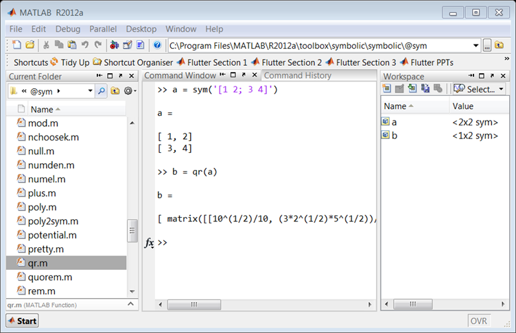
Approach 3: The MathWorks do not recommend that you modify your MATLAB install. However for completeness, it is possible to add a new ‘method’ to the sym class by dropping your function into the sym class folder.  For MATLAB 2012a on Windows, this folder is at

C:\Program Files\MATLAB\R2012a\toolbox\symbolic\symbolic\@sym

For the sake of illustration, here is a simplified implementation. Call it qr.m

function result = qr( this )
  result = feval(symengine,'linalg::factorQR', this);
end

Pros: Functions saved to a class folder take precedence over built in functionality, which means that MATLAB will always use your qr method for sym objects.

Cons: If you share code which uses this functionality, it won’t run on someone’s computer unless they update their sym class folder with your qr code. Additionally, if a new method is added to a class it may shadow the behaviour of other MATLAB functionality and lead to unexpected behaviour in Symbolic Toolbox.

Approach 4: For more of an object-oriented approach it is possible to sub-class the sym class, and add a new qr method.

classdef mySym < sym

    methods
        function this = mySym(arg)
            this = this@sym(arg);
        end

        function result = qr( this )
            result = feval(symengine,'linalg::factorQR', this);
        end
    end

end

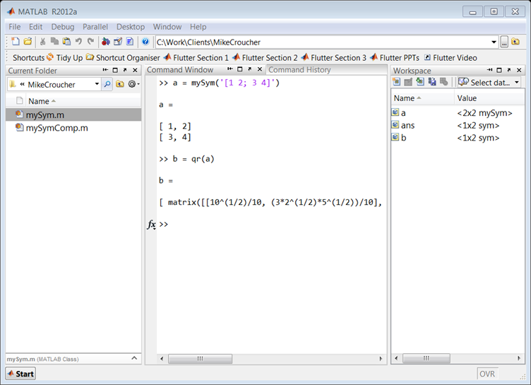
Pros: Your change can be shipped with your code and it will work on a client’s computer without having to change the sym class.

Cons: When calling superclass methods on your mySym objects (such as sin(mySym1)), the result will be returned as the superclass unless you explicitly redefine the method to return the subclass.

N.B. There is a lot of literature which discusses why inheritance (subclassing) to augment a class’s behaviour is a bad idea. For example, if Symbolic Toolbox developers decide to add their own qr method to the sym API, overriding that function with your own code could break the system. You would need to update your subclass every time the superclass is updated. This violates encapsulation, as the subclass implementation depends on the superclass. You can avoid problems like these by using composition instead of inheritance.

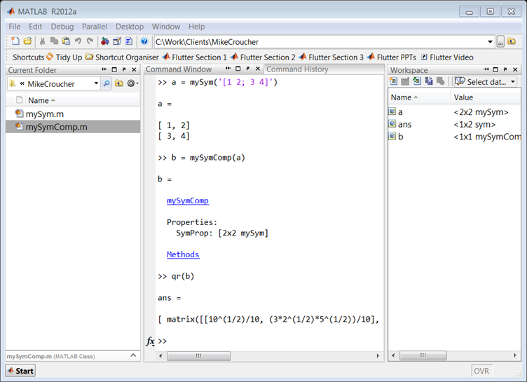
Approach 5: You can create a new sym class by using composition, but it takes a little longer than the other approaches. Essentially, this involves creating a wrapper which provides the functionality of the original class, as well as any new functions you are interested in.

classdef mySymComp

    properties
        SymProp
    end

    methods
        function this = mySymComp(symInput)
            this.SymProp = symInput;
        end

        function result = qr( this )
            result = feval(symengine,'linalg::factorQR', this.SymProp);
        end
    end

end

Note that in this example we did not add any of the original sym functions to the mySymComp class, however this can be done for as many as you like. For example, I might like to use the sin method from the original sym class, so I can just delegate to the methods of the sym object that I passed in during construction:

classdef mySymComp

    properties
        SymProp
    end

    methods
        function this = mySymComp(symInput)
            this.SymProp = symInput;
        end

        function result = qr( this )
            result = feval(symengine,'linalg::factorQR', this.SymProp);
        end

        function G = sin(this)
            G = mySymComp(sin(this.SymProp));
        end
    end

end

Pros: The change is totally encapsulated, and cannot be broken save for a significant change to the sym api (for example, the MathWorks adding a qr method to sym would not break your code).

Cons: The wrapper can be time consuming to write, and the resulting object is not a ‘sym’, meaning that if you pass a mySymComp object ‘a’ into the following code:

isa(a, 'sym')

MATLAB will return ‘false’ by default.

In a recent article, Citing software in research papers, I discussed how to cite various software packages.  One of the commentators suggested that I should contact The Mathworks if I wanted to know how to cite MATLAB.  I did this and asked for permission to blog the result.  This is what they suggested:

To cite MATLAB (and in this case a toolbox) you can use this:

MATLAB and Statistics Toolbox Release 2012b, The MathWorks, Inc., Natick, Massachusetts, United States.

This is the format prescribed by both the Chicago Manual of Style and the Microsoft Manual of Style. If you use a different style guide, you may apply a different format, but should observe the capitalization shown above, and include the appropriate release number. If the MathWorks release number (in the format YYYYa or YYYYb) is not readily available, you can use the point release numbers for the software, as in:

MATLAB 8.0 and Statistics Toolbox 8.1, The MathWorks, Inc., Natick, Massachusetts, United States.

Thanks to The Mathworks for allowing me to reproduce this communication here at WalkingRandomly.

xkcd is a popular webcomic that sometimes includes hand drawn graphs in a distinctive style.  Here’s a typical example

In a recent Mathematica StackExchange question, someone asked how such graphs could be automatically produced in Mathematica and code was quickly whipped up by the community.  Since then, various individuals and communities have developed code to do the same thing in a range of languages.  Here’s the list of examples I’ve found so far

• xkcd style graphs in Mathematica. There is also a Wolfram blog post on this subject.
• xkcd style graphs in R. A follow up blog post at vistat.
• xkcd style graphs in LaTeX
• xkcd style graphs in Python using matplotlib
• xkcd style graphs in MATLAB. There is now some code on the File Exchange that does this with your own plots.
• xkcd style graphs in javascript using D3
• xkcd style graphs in Euler
• xkcd style graphs in Fortran

Any I’ve missed?

MATLAB Mobile has been around for Apple devices for a while now but Android users have had to make do with third party alternatives such as MATLAB Commander and MLConnect.  All that has now changed with the release of MATLAB Mobile for Android.

MATLAB Mobile is NOT MATLAB running on your phone

While MATLAB Mobile is a very nice and interesting product, there is one thing you should get clear in your mind– this is not a full version of MATLAB on your phone or Tablet.  MATLAB Mobile is essentially a thin client that connects to an instance of MATLAB running on your desktop or The Mathworks Cloud.  In other words, it doesn’t work at all if you don’t have a network connection or a licensed copy of MATLAB.

What if you do want to run MATLAB code directly on your phone?

While it is unlikely that we’ll see a full version of MATLAB compiled for Android devices any time soon, Android toting MATLABers have a couple of other options available to them in addition to MATLAB Mobile.

• Octave for Android Octave is a free, open source alternative to MATLAB that can run many .m file scripts and functions.  Corbin Champion has ported it to Android and although it is still a work in progress, it works very well.
• Mathmatiz – Small and light, this free app understands a subset of the MATLAB language and can do basic plotting.
• Addi – Much smaller and less capable than Octave for Android, this is Corbin Champion’s earlier attempt at bringing a free MATLAB clone to Android.  It is based on the Java library, JMathLib.

Simulink from The Mathworks is widely used in various disciplines.  I was recently asked to come up with a list of alternative products, both free and commercial.

Here are some alternatives that I know of:

• MapleSim – A commercial Simuink replacement from the makers of the computer algebra system, Maple
• OpenModelica -An open-source Modelica-based modeling and simulation environment intended for industrial and academic usage
• Wolfram SystemModeler – Very new commercial product from the makers of Mathematica.  Click here for Wolfram’s take on why their product is the best.
• xcos – This free Simulink alternative comes with Scilab.

I plan to keep this list updated and, eventually, include more details.  Comments, suggestions and links to comparison articles are very welcome.  If you have taught a course using one of these alternatives and have experiences to share, please let me know.  Similarly for anyone who was switched (or attempted to switch) their research from Simulink.  Either comment to this post or contact me directly.

I’ve nothing against Simulink but would like to get a handle on what else is out there.

I felt like playing with Julia and MATLAB this Sunday morning.  I found some code that prices European Options in MATLAB using Monte Carlo simulations over at computeraidedfinance.com and thought that I’d port this over to Julia.  Here’s the original MATLAB code

function V = bench_CPU_European(numPaths)
%Simple European
steps = 250;
r = (0.05);
sigma = (0.4);
T = (1);
dt = T/(steps);
K = (100);

S = 100 * ones(numPaths,1);

for i=1:steps
 rnd = randn(numPaths,1);
 S = S .* exp((r-0.5*sigma.^2)*dt + sigma*sqrt(dt)*rnd);
end
V = mean( exp(-r*T)*max(K-S,0) )

I ran this a couple of times to see what results I should be getting and how long it would take for 1 million paths:

tic;bench_CPU_European(1000000);toc
V =
   13.1596
Elapsed time is 6.035635 seconds.
>> tic;bench_CPU_European(1000000);toc
V =
   13.1258
Elapsed time is 5.924104 seconds.
>> tic;bench_CPU_European(1000000);toc
V =
   13.1479
Elapsed time is 5.936475 seconds.

The result varies because this is a stochastic process but we can see that it should be around 13.1 or so and takes around 6 seconds on my laptop. Since it’s Sunday morning, I am feeling lazy and have no intention of considering if this code is optimal or not right now. I’m just going to copy and paste it into a julia file and hack at the syntax until it becomes valid Julia code. The following seems to work

function bench_CPU_European(numPaths)

steps = 250
r = 0.05
sigma = .4;
T = 1;
dt = T/(steps)
K = 100;

S = 100 * ones(numPaths,1);

for i=1:steps
 rnd = randn(numPaths,1)
 S = S .* exp((r-0.5*sigma.^2)*dt + sigma*sqrt(dt)*rnd)
end
V = mean( exp(-r*T)*max(K-S,0) )
end

I ran this on Julia and got the following

julia> tic();bench_CPU_European(1000000);toc()
elapsed time: 36.259000062942505 seconds
36.259000062942505

julia> bench_CPU_European(1000000)
13.114855104505445

The Julia code appears to be valid, it gives the correct result of 13.1 ish but at 36.25 seconds is around 6 times slower than the MATLAB version.  The dog needs walking so I’m going to think about this another time but comments are welcome.

Update (9pm 7th October 2012):   I’ve just tried this Julia code on the Linux partition of the same laptop and 1 million paths took 14 seconds or so:

tic();bench_CPU_European(1000000);toc()
elapsed time: 14.146281957626343 seconds

I built this version of Julia from source and so it’s at the current bleeding edge (version 0.0.0+98589672.r65a1 Commit 65a1f3dedc (2012-10-07 06:40:18). The code is still slower than the MATLAB version but better than the older Windows build

Update: 13th October 2012

Over on the Julia mailing list, someone posted a faster version of this simulation in Julia

function bench_eu(numPaths)
    steps = 250
    r = 0.05
    sigma = .4;
    T = 1;
    dt = T/(steps)
    K = 100;

    S = 100 * ones(numPaths,1);

    t1 = (r-0.5*sigma.^2)*dt
    t2 = sigma*sqrt(dt)
    for i=1:steps
        for j=1:numPaths
            S[j] .*= exp(t1 + t2*randn())
        end
    end

    V = mean( exp(-r*T)*max(K-S,0) )
end

On the Linux partition of my test machine, this got through 1000000 paths in 8.53 seconds, very close to the MATLAB speed:

julia> tic();bench_eu(1000000);toc()
elapsed time: 8.534484148025513 seconds

It seems that, when using Julia, one needs to unlearn everything you’ve ever learned about vectorisation in MATLAB.

Update: 28th October 2012

Members of the Julia team have been improving the performance of the randn() function used in the above code (see here and here for details).  Using the de-vectorised code above, execution time for 1 million paths in Julia is now down to 7.2 seconds on my machine on Linux.  Still slower than the MATLAB 2012a implementation but it’s getting there.  This was using Julia version  0.0.0+100403134.r0999 Commit 099936aec6 (2012-10-28 05:24:40)

tic();bench_eu(1000000);toc()
elapsed time: 7.223690032958984 seconds
7.223690032958984

• Laptop model: Dell XPS L702X
• CPU:Intel Core i7-2630QM @2Ghz software overclockable to 2.9Ghz. 4 physical cores but total 8 virtual cores due to Hyperthreading.
• RAM: 8 Gb
• OS: Windows 7 Home Premium 64 bit and Ubuntu 12.04
• MATLAB: 2012a
• Julia: Original windows version was Version 0.0.0+94063912.r17f5, Commit 17f50ea4e0 (2012-08-15 22:30:58).  Several versions used on Linux since, see text for details.