May 10th, 2011 | Categories: Carnival of Math, general math | Tags:

I do the administration for the Carnival of Mathematics and am very happy to announce that the 77th edition has been published over at Jost a Mon.  If you are unsure what a Math carnival is then check out my introductory article or just read some past editions from either the Carnival of Math itself or its sister publication, Math Teachers at Play which is run by Denis of Let’s Play Math fame.

The next Carnival of Math is scheduled to be hosted over at JimWilder.com and the submission form for articles is open now.  If you’d like to host a future carnival of math on your blog or website then please contact me for further details.

May 10th, 2011 | Categories: iPad, just for fun | Tags:

A while ago I wrote an article on comparing mobile phones with ancient supercomputers and today I learned that Jack Dongarra has run his Linpack benchmark on the iPad 2 and discovered that it has enough processing power to rival the Cray 2; the most powerful supercomputer in the world back in 1985.  According to Jack, the iPad 2 is so powerful that it would have stayed in the top 500 list of world’s most powerful super computers until 1994.  That’s a lot of power!

Other iPad articles on WalkingRandomly

May 6th, 2011 | Categories: CUDA, GPU, Maple, math software, mathcad, mathematica, matlab, OpenCL, parallel programming | Tags:

Updated January 4th 2011

It is becoming increasingly common for programmers to make use of GPUs (Graphical Processing Units) to speed up their programs substantially.  There are three major low-level programming libraries that allow you to do this in languages such as C; namely CUDA, OpenCL and Microsoft DirectCompute.  Of these three, CUDA is the most developed but it only works on Nvidia graphics cards.

I am often asked if the major commercial math packages support GPU computing and I find myself writing the same summary email over and over again.  So, here is a very brief breakdown of what is currently on offer.  I plan to expand the information contained in this page over time so if you have any information about GPU computing in these packages then let me know.

MATLAB

Core MATLAB contains no support for GPU computing but several organizations (including The Mathworks themselves) have produced add-on toolboxes that add such support:

  • Jacket – This is a product from a company called AccelerEyes and is possibly the most advanced and well developed GPU solution for MATLAB currently available.  As of version 2.0 it supports both OpenCL and CUDA frameworks.
  • The Mathworks’ Parallel Computing Toolbox (PCT) – If you want to do your MATLAB GPU computing the officially supported way then this is the product you need.  As a bonus, it also allows you to make better use of the multicore processor that almost certainly resides in your machine.  Like many of the offerings on this page, only the CUDA framework is supported so you are out of luck if you don’t have an NVidia graphics card.  Even if you do have an NVidia graphics card then you still might be out of luck since the PCT only supports cards that have compute level 1.3 or above (i.e. double precision only).
  • CULA is a set of GPU-accelerated linear algebra libraries utilizing the NVIDIA CUDA parallel computing architecture and it has a MATLAB interface.
  • GPUmat – This product is completely free but is less developed than the commercial offerings above.  Again. it is CUDA only
  • OpenCL toolbox – The only OpenCL solution for MATLAB I could find.  It is free but development seems to have stalled.

Mathematica

Mathematica 8 has support for both CUDA and OpenCL built in so no need for any add-ons.  Furthermore, it supports both single and double precision GPUs so you can experiment with GPU computing on older, cheaper cards.

Maple

Maple has had some CUDA-only GPU support since version 14.  On the face of it, the CUDA package only appears to contain one accelerated function–Matrix-Matrix multiplication– but when you load this function it accelerates many functions that use matrix-matrix multiply internally.  I’ve never found a definitive list of such functions though.

Mathcad

Mathcad 15 and Mathcad Prime have no support for GPU enhanced computing.

May 1st, 2011 | Categories: math software, Month of Math Software | Tags:

Welcome to the slightly delayed 4th edition of ‘A Month of Math Software’.  If you have some math software news that you’d like including in a future edition then let me know.  Previous articles can be found in the archive.

News

Wolfram Research have acquired a company called MathCore Engineering AB – http://www.mathcore.com/.  The practical upshot of this is that we can expect future Mathematica versions to contain Simulink-like functionality.  Wolfram’s press-release is at http://www.wolfram.com/news/mathcoreaquired.html and Stephen Wolfram spoke about this at http://blog.wolfram.com/2011/03/30/launching-a-new-era-in-large-scale-systems-modeling/.

Commercial releases

MATLAB 2011a was released by The Mathworks earlier this month.  There have been a lot of changes around various toolboxes along with the usual performance enhancements and so on.  I’ll be doing a write up of it at some point but, for now, here are the release highlights .

Maplesoft’s Maple has seen a new major version.  Maple 15 has got lots of new goodies.  Check them out at http://www.maplesoft.com/products/maple/new_features/ which includes lots of examples of how Maple 15 is better than previous versions (and, in some cases, the competition).

The popular data analysis and plotting application, Origin, has seen an upgrade to version 8.5.1.  The what’s new list is at http://www.originlab.com/index.aspx?go=Products/Origin&PID=1750 This package is a firm favourite of users at my workplace, The University of Manchester.  It’s just a shame that it is Windows only.  Ho hum!

HSL 2011 has been released; the first major release in 4 years.  From the website: “HSL (formerly the Harwell Subroutine Library) is a collection of state-of-the-art packages for large-scale scientific computation written and developed by the Numerical Analysis Group at the STFC Rutherford Appleton Laboratory and other experts.” Although this is a commercial library, it is free for academic use.

I’ve been writing ‘A month of Math Software’ for four months now and you can always rely on the commercial computational algebra system, Magma, to supply us with some news.  The v2.17-6 release change log is at http://magma.maths.usyd.edu.au/magma/releasenotes/2/17/7/

Open Source releases

One of the most powerful statistical programming languages in existence, R, has seen a new major release.  Version 2.13 was released on April 13th.  One of the biggest new developments is a new bytecode compiler for R which has been demonstrated and benchmarked over at Thinking Inside the Box.  The huge list of changes is available in the NEWS file.

Maxima, the free open source computer algebra system for Windows, Mac and Linux, was upgraded to version 5.24 earlier this month.  The changelog is available at http://maxima.cvs.sourceforge.net/viewvc/maxima/maxima/ChangeLog-5.24

April 28th, 2011 | Categories: general math, math software, mathematica, programming | Tags:

Last month I published an article that included an interactive mathematical demonstration powered by Wolfram’s new CDF (Computable Document Format) player.  These demonstrations work on many modern web-browsers including Internet Explorer 8 and Firefox 3.6.  So, how do you go about adding them to your own websites?

What you need

  • Mathematica 8.0.1 or above to create demonstrations.  Viewers of your demonstration only need the free CDF player for their platform.
  • A modern browser such as Internet Explorer 8, Firefox 3.6 or Safari 5.
  • Basic knowledge of HTML, uploading files to a webserver etc. If you maintain a blog or similar then you almost certainly know enough

Our aim is the following, very simple, interactive demonstration.

Series demo

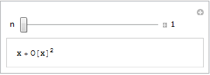
If all you see is a static image then you do not have the CDF player or Mathematica 8 correctly installed. Alternatively, you are using an unsupported platform such as Linux, iOS or Android.

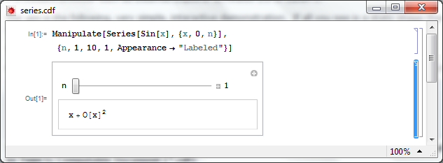
Step 1 – Create the .cdf file

Fire up Mathematica, type in and evaluate the following code.  You should get an applet similar to the one above.

Manipulate[
 Series[Sin[x], {x, 0, n}]
 , {n, 1, 10, 1, Appearance -> "Labeled"}
 ]

Save it as a .cdf file called series.cdf by clicking on File->Save as  — Give it the File Name series.cdf and change the Save as Type to Computable Document (*.cdf)

Save as CDF

Step 2 – Get a static screenshot

Not everyone is going to have either Mathematica 8 or the free CDF player installed when they visit your website so we need to give them something to look at.  So, lets give them a static image of the Manipulate applet.  As a bonus, this will act as a place holder for the interactive version for those who do have the requisite software.

Open series.cdf in Mathematica and left click on the bracket surrounding the manipulate (see below). Click on Cell->Convert To->Bitmap. Then click on File->Save Selection As . Make sure you change .pdf to something more sensible such as .png

Don’t save your .cdf file at this point or it won’t be interactive. Re-evaluate the code again to get back your interactive Manipulate.

Here’s one I made earlier – series.png

Select Manipulate

Step 4 – Hide the source code

In this particular instance, I don’t want the user to see the source code.  So, lets sort that out.

  • Open series.cdf in Mathematica if you haven’t already and make sure that the Manipulate is evaluated.
  • Left click on the inner cell bracket surrounding the Manipulate source code only and click on Cell->Cell Properties and un-tick Open

Step 5 – Hide the cell brackets

Those blue brackets at the far right of the Mathematica notebook are called the Cell brackets and I don’t want to see them on my web site as they make the applet look messy.

  • Open series.cdf in Mathematica if you haven’t already
  • Open the option inspector: Edit->Preferences->Advanced->Open Option Inspector
  • Ensure Show option values is set to “series.cdf” and that they are sorted by category. Click on Apply.
  • Click on Cell Options-> Display options and in the right hand pane set ShowCellBracket to False
  • Click Apply

Before you save series.cdf ensure that the applet is interactive and not a static bitmap.  If it isn’t interactive then click on Evaluation->Evaluate notebook to re-evaluate the (now hidden) source code.  Also ensure that there is nothing but the applet anywhere else in the notebook.

Step 6 – Get interactive on your website

Upload series.png and series.cdf to your server.  The next thing we need to do is get the static image into our webpage. Here’s what the HTML might look like

<img id="Series_applet" src="series.png" alt="Series demo" />

Obviously, you’ll need to put the full path to series.png on your server in this piece of code. The only thing that is different to the way you might usually use the img tag is that it includes an id; in this case it is Series_applet. We’ll make use of this later.

The magic happens thanks to a small javascript applet called the CDF javascript plugin. Version one is at http://www.wolfram.com/cdf-player/plugin/v1.0/cdfplugin.js and that’s the one I’ll be using here. Here’s the code which needs to be placed before the img tag in your HTML file.

<script src="http://www.wolfram.com/cdf-player/plugin/v1.0/cdfplugin.js"
type="text/javascript"></script><script type="text/javascript">// <![CDATA[
var cdf = new cdf_plugin();
cdf.addCDFObject("Series_applet", "series.cdf", 403,109);
// ]]></script>

The only line you’ll need to change if you use this for anything else is

cdf.addCDFObject("Series_applet", "series.cdf", 403,109);

where Series_applet is the id of the image we wish to replace and series.cdf is the cdf file we want to replace it with. The numbers 403,109 are the dimensions of the applet.  These will not be the same as the .png file as the dimensions of the .cdf file are slightly larger.  I used trial and error to determine what they should be as I haven’t come up with a better way yet (suggestions welcomed).

So that’s it for now. Hope this mini-tutorial was useful. Let me know if you upload any demonstrations to your own website or if you have any comments, questions or problems.

Update (6th June 2011)

Thanks to ‘Paul’ in the comments section, I have discovered that this mechanism won’t work for .cdf files that Wolfram deem are unsafe.  According to Paul the definition of unsafe is as follows:

Dynamic content is considered unsafe if it:

  • uses File operations
  • uses interprocess communication via MathLink Mathematica Functions
  • uses JLink or NETLink
  • uses Low-Level Notebook Programming
  • uses data as code by Converting between Expressions and Strings
  • uses Namespace Management
  • uses Options Management
  • uses External Programs
April 11th, 2011 | Categories: general math, math software, walking randomly | Tags:

I love mathematics and I also love gadgets so you’d think that I’d be overjoyed to learn that there are a couple of new graphical calculators on the block.  You’d be wrong!

Late last year, Casio released the Prizm colour graphical calculator.  It costs $130 and its spec is pitiful:

  • 216*384 pixel display with 65,536 colours
  • 16Mb memory
  • The CPU is a SuperH 3 running at 58Mhz (according to this site)

Casio Prizm.

More recently, Texas Instruments countered with its color offering, the TI-NSpire CX CAS.  This one costs $162 (source) and its specs are also a bit on the weak side but quite a bit higher than the Casio.

  • 320*240 pixels with 65,536 colours
  • 100Mb memory
  • CPU? I have no idea.  Can anyone help?

If you are into retro-computing then those specs might appeal to you but they leave me cold. They are slow with limited memory and the ‘high-resolution’ display is no such thing. For $100 dollars more than the NSpire CX CAS I could buy a netbook and fill it with cutting edge mathematical software such as Octave, Scilab, SAGE and so on.  I could also use it for web browsing,email and a thousand other things.

I (and many students) also have  mobile phones with hardware that leave these calculators in the dust.  Combined with software such as Spacetime or online services such as Wolfram Alpha, a mobile phone is infinitely more capable than these top of the line graphical calculators.

They also only ever seem to be used in schools and colleges.  I spend a lot of time working with engineers, scientists and mathematicians and I hardly ever see a calculator such as the Casio Prizm or TI NSpire on their desks.  They tend to have simple calculators for everyday use and will turn to a computer for anything more complicated such as plotting a graph or solving equations.

One argument I hear for using these calculators is ‘They are limited enough to use in exams.‘  Sounds sensible but then I get to thinking ‘Why are we teaching a generation of students to use crippled technology?‘ Why not go the whole hog and ban ALL technology in exams?  Alternatively, supply locked down computers for exams that limit the software used by students.  Surely we need experts in useful technology, not crippled technology?

So, I don’t get it.  Why do so many people advocate the use of these calculators?  They seem pointless!  Am I missing something?  Comments welcomed.

Update 1: I’ve been slashdotted!  Check out the slashdot article for more comments.

Update 2: My favourite web-comic, xkcd, covered this subject a while ago.

Other posts you may find useful / interesting

April 10th, 2011 | Categories: Carnival of Math | Tags:

Welcome to the very late 76th carnival of Maths.  As per tradition, lets start with the trivia.  76 is an automorphic number , can be written as a sum of three squares (2^2+6^2+6^2) and is the 9th Lucas number.
Spirit of 76

Every now and then I get asked the question ‘Eigenvectors….so what are they good for?’  I’ve got a few stock answers but Language Log’s Mark Liberman goes the extra mile when he considers how they might have been used in Cinderella and goes on to discuss how they are used in linguistics.  Are you suitably intrigued?  Check it out in  Eigenfeet, eigenfaces, eigenlinguistics, …

If you have worked on the classification of multivariate data then you may well have heard of or used the Mahalanobis distance (I came across it for the first time when working with MATLAB’s pdist function).  It turns out that this commonly used metric has rather surprising origins!  Read all about it in Anthropometry and Anglo-Indians over at Jost a Mon.

March 14th is, of course, Pi day and several bloggers have written something about everyone’s favouburite irrational number.  Carnival regular, John D. Cook, brings us A Ramanujan series for calculating pi, 360 has The Difference and Qiaochu Yuan counters with Pi is still wrong.  Finally, madkane brings us a Pi day limerick.

Over at God Plays Dice, Michael Lugo brings us A street-fighting approach to the variance of a hypergeometric random variable and some of Denise’s favourite math websites have gone AWOL over at Let’s Play Math.  Can you help her find them?

Peter Rowlett asked Twitter for links to enthuse people about mathematics. Here are the answers.  Finally, Guillermo Bautista gives us an example of the epsilon-delta definition of limits.

Your Carnival needs you

The Carnival of Math desperately needs people to write and host future editions.  If you have a math related blog and would like a bucket-load of extra traffic then contact me for more information.

April 7th, 2011 | Categories: Guest posts, programming | Tags:

A couple of weeks ago my friend and colleague, Ian Cottam, wrote a guest post here at Walking Randomly about his work on interfacing Dropbox with the high throughput computing software, Condor.  Ian’s post was very well received and so he’s back; this time writing about a very different kind of project.  Over to Ian.

Natural Scientists: their very big output files – and a tale of diffs by Ian Cottam

I’ve noticed that natural scientists (as opposed to computer scientists) often write, or use, programs that produce masses of output, usually just numbers. It might be the final results file or, often, some intermediate test results.

Am I being a little cynical in thinking that many users glance – ok, carefully check – a few of these thousands (millions?) of numbers and then delete the file? Let’s assume such files are really needed. A little automation is often added to the process by having a baseline file and running a program to show you the differences between it and your latest output (assuming wholesale changes are not the norm).

One of the popular difference programs is the Unix diff command . (I’ve been using it since the 1970s.) It popularised the idea of showing minimal differences between two text files (and, later, binary ones too). There are actually a few algorithms for doing minimal difference computation, and GNU diff, for example, uses a different one from the original Bell Labs version. They all have one thing in common: to achieve minimal difference computation the two files being compared must be read into main memory (aka RAM). Back in the 1970s, and on my then department’s PDP-11/40, this restricted the size of the files considerably; not that we noticed much as everything was 16bit and “small was beautiful”. GNU diff, on modern machines, can cope with very big files, but still chokes if your files, in aggregate, approach the gigabyte range.

(As a bit of an aside: a major contribution of all the GNU tools, over what we had been used to from the Unix pioneers at Bell Labs, was that they removed all arbitrary size restrictions; the most common and frustrating one being the length of text lines.)

Back to the 1970s again: Bell Labs did know that some files were too big to compare with diff , and they also shipped: diffh. The h stands for halfhearted. Diffh does not promise minimal differences, but can be very good for big files with occasional differences. It uses a pass over the files using a simple ‘sliding window’ heuristic approach (the other word that the h is sometimes said to stand for). You can still find an old version of diffh on the Internet. However, it ‘gives up’ rather easily and you may have to spend some time modifying it for, e.g., 64 bit ints and pointers, as well as for compiling with modern C compilers. Other tools exist that can compare enormous files, but they don’t produce readable output in diff’s pleasant format.

A few years back, when a user at the University of Manchester asked for help with the ‘diff – files too big/ out of memory’ problem, I wrote a modern version that I called idiffh (for Ian’s diffh). My ground rules were:

  • Work on any text files on any operating system with a C compiler
  • Have no limits on, e.g., line lengths or file size
  • Never ‘give up’ if the going gets tough (i.e. when the files are very different)

You won’t find this with the GNU collection as they like to write code to the Unix interface and I like to write to the C standard I/O interface (see the first bullet point above).

An interesting implementation detail is that it uses random access to the files directly, relying on the operating system’s cache of file blocks to make this tolerably efficient. Waiting a minute or two to compare gigabyte sized files is usually acceptable.

As the comments in the code say, you can get some improvements by conditional compilation on Unix systems and especially on BSD Systems (including Apple Macs), but you can compile it straight, without such, on Windows and other platforms.

If you would like to try idffh out you can download it here.

March 29th, 2011 | Categories: math software, Month of Math Software | Tags:

Welcome to the March 2011 edition of A Month of Math Software (MMS) where I take you on a brief tour of new things in the world of mathematical software.  If you like what you see then you may also be interested in last month’s edition and possibly January’s too. If I’ve missed anything then contact me and let me know.

Commercial releases

A minor update to Mathematica has been released.  Version 8.0.1 contains bug fixes and enhancements and a short list of these is available at http://www.wolfram.com/mathematica/quick-revision-history.html

Another month, another Magma release.  See what’s new in 2.17-6 here.

Open source releases

Version 5.3.1 of Scilab, a superb free MATLAB-like environment, has been released.  Check out http://www.scilab.org/en/products/scilab/download/5.3.1/whatsnew to see what’s new.

A new minor release (version 4.4.3) of GNUPLOT, a popular open-source plotting package, is now available.  The changelog is available at http://www.gnuplot.info/announce.4.4.3

SAGE, the open-source mathematics package based on Python, has seen a new minor release.  Version 4.6.2 was released just after I published February’s edition of MMS so I’ve included it here.  For a list of all things new see this thread.

Version 1.10.14 of Gnumeric, a free alternative to Excel, has been released.  Lots of new goodness listed at http://projects.gnome.org/gnumeric/announcements/1.10/gnumeric-1.10.14.shtml

Version 12 of EuMaT (Euler Math Toolbox) has been released but I can’t find a changelog (update: changelog is here) .  If you’ve never used this software before then it’s a bit MATLAB-like and uses Maxima for symbolic stuff.

Euler Math Toolbox

GP-GPU (General Purpose Graphics Processing Units) related news, tutorials and releases

NVIDIA have released version 4.0 of their CUDA toolkit.

Jacket, arguably the most advanced GPU-accelerated toolbox for MATLAB currently available, has been updated to version 1.7  Check out the release notes to see what’s been added.

PGI insider have an article called Using GPU-enabled Math Libraries with PGI Fortran which covers GPU accelerated libraries such as CUBLAS, CULA and MAGMA.

Odds and ends

Version 4.0 of the free MATLAB toolbox, Chebfun, has been released.  Chebfun is a collection of algorithms, and a software system in object-oriented MATLAB, which extends familiar powerful methods of numerical computation involving numbers to continuous or piecewise-continuous functions.  Chebfun is a very interesting project as can be seen from the wide array of examples.

March 26th, 2011 | Categories: matlab, programming | Tags:

My passions include mathematics, mathematical software and gadgets.  So, I instantly fell in love with the LED Cube.  The programming was done in C but MATLAB was used for some of the prototyping.

If you prefer something more physical then how about the MATLAB-controlled 3D function machine?

MATLAB function machine

Perhaps you prefer a more retro, aural kind of a vibe? MATLAB-controlled carol singing dot-matrix printers anyone?

Update: In case it isn’t clear.  None of the three projects above are my work, they are other people’s work!  I just think they are cool!

Want to have a play?
If you’d like to use MATLAB as a way into physical computing then maybe the following resources will help you.  I don’t think that they were used in the projects above but if I were to start playing with such things then I probably begin with one of these.