Walking Randomly

Computing Eigenvalues without balancing in Python using the NAG library

December 17th, 2013

In a recent Stack Overflow query, someone asked if you could switch off the balancing step when calculating eigenvalues in Python. In the document A case where balancing is harmful, David S. Watkins describes the balancing step as ‘the input matrix A is replaced by a rescaled matrix A* = D^-1AD, where D is a diagonal matrix chosen so that, for each i, the ith row and the ith column of A* have roughly the same norm.’

Such balancing is usually very useful and so is performed by default by software such as MATLAB or Numpy. There are times, however, when one would like to switch it off.

In MATLAB, this is easy and the following is taken from the online MATLAB documentation

A = [ 3.0     -2.0      -0.9     2*eps;
     -2.0      4.0       1.0    -eps;
     -eps/4    eps/2    -1.0     0;
     -0.5     -0.5       0.1     1.0];

[VN,DN] = eig(A,'nobalance')
VN =

    0.6153   -0.4176   -0.0000   -0.1528
   -0.7881   -0.3261         0    0.1345
   -0.0000   -0.0000   -0.0000   -0.9781
    0.0189    0.8481   -1.0000    0.0443

DN =
    5.5616         0         0         0
         0    1.4384         0         0
         0         0    1.0000         0
         0         0         0   -1.0000

At the time of writing, it is not possible to directly do this in Numpy (as far as I know at least). Numpy’s eig command currently uses the LAPACK routine DGEEV to do the heavy lifting for double precision matrices. We can see this by looking at the source code of numpy.linalg.eig where the relevant subsection is

lapack_routine = lapack_lite.dgeev
        wr = zeros((n,), t)
        wi = zeros((n,), t)
        vr = zeros((n, n), t)
        lwork = 1
        work = zeros((lwork,), t)
        results = lapack_routine(_N, _V, n, a, n, wr, wi,
                                  dummy, 1, vr, n, work, -1, 0)
        lwork = int(work[0])
        work = zeros((lwork,), t)
        results = lapack_routine(_N, _V, n, a, n, wr, wi,
                                  dummy, 1, vr, n, work, lwork, 0)

My plan was to figure out how to tell DGEEV not to perform the balancing step and I’d be done. Sadly, however, it turns out that this is not possible. Taking a look at the reference implementation of DGEEV, we can see that the balancing step is always performed and is not user controllable–here’s the relevant bit of Fortran

*     Balance the matrix
*     (Workspace: need N)
*
      IBAL = 1
      CALL DGEBAL( 'B', N, A, LDA, ILO, IHI, WORK( IBAL ), IERR )

So, using DGEEV is a dead-end unless we are willing to modifiy and recompile the lapack source — something that’s rarely a good idea in my experience. There is another LAPACK routine that is of use, however, in the form of DGEEVX that allows us to control balancing. Unfortunately, this routine is not part of the numpy.linalg.lapack_lite interface provided by Numpy and I’ve yet to figure out how to add extra routines to it.

I’ve also discovered that this functionality is an open feature request in Numpy.

Enter the NAG Library

My University has a site license for the commercial Numerical Algorithms Group (NAG) library. Among other things, NAG offers an interface to all of LAPACK along with an interface to Python. So, I go through the installation and do

import numpy as np
from ctypes import *
from nag4py.util import Nag_RowMajor,Nag_NoBalancing,Nag_NotLeftVecs,Nag_RightVecs,Nag_RCondEigVecs,Integer,NagError,INIT_FAIL
from nag4py.f08 import nag_dgeevx

eps = np.spacing(1)
np.set_printoptions(precision=4,suppress=True) 

def unbalanced_eig(A):
    """
    Compute the eigenvalues and right eigenvectors of a square array using DGEEVX via the NAG library.
    Requires the NAG C library and NAG's Python wrappers http://www.nag.co.uk/python.asp
    The balancing step that's performed in DGEEV is not performed here.
    As such, this function is the same as the MATLAB command eig(A,'nobalance')

    Parameters
    ----------
    A : (M, M) Numpy array
        A square array of real elements.

        On exit: 
        A is overwritten and contains the real Schur form of the balanced version of the input matrix .

    Returns
    -------
    w : (M,) ndarray
        The eigenvalues
    v : (M, M) ndarray
        The eigenvectors

    Author: Mike Croucher (www.walkingrandomly.com)
    Testing has been mimimal
    """

    order = Nag_RowMajor
    balanc = Nag_NoBalancing
    jobvl = Nag_NotLeftVecs
    jobvr = Nag_RightVecs
    sense = Nag_RCondEigVecs

    n = A.shape[0]
    pda = n
    pdvl = 1

    wr = np.zeros(n)
    wi = np.zeros(n)

    vl=np.zeros(1);
    pdvr = n
    vr = np.zeros(pdvr*n)

    ilo=c_long(0)
    ihi=c_long(0)

    scale = np.zeros(n)
    abnrm = c_double(0)
    rconde = np.zeros(n)
    rcondv = np.zeros(n)

    fail = NagError()
    INIT_FAIL(fail)

    nag_dgeevx(order,balanc,jobvl,jobvr,sense, 
               n, A.ctypes.data_as(POINTER(c_double)), pda, wr.ctypes.data_as(POINTER(c_double)),
               wi.ctypes.data_as(POINTER(c_double)),vl.ctypes.data_as(POINTER(c_double)),pdvl, 
               vr.ctypes.data_as(POINTER(c_double)),pdvr,ilo,ihi, scale.ctypes.data_as(POINTER(c_double)),
               abnrm, rconde.ctypes.data_as(POINTER(c_double)),rcondv.ctypes.data_as(POINTER(c_double)),fail)

    if all(wi == 0.0):
            w = wr
            v = vr.reshape(n,n)
    else:
            w = wr+1j*wi
            v = array(vr, w.dtype).reshape(n,n)

    return(w,v)

Define a test matrix:

A = np.array([[3.0,-2.0,-0.9,2*eps],
          [-2.0,4.0,1.0,-eps],
          [-eps/4,eps/2,-1.0,0],
          [-0.5,-0.5,0.1,1.0]])

Do the calculation

(w,v) = unbalanced_eig(A)

which gives

(array([ 5.5616,  1.4384,  1.    , -1.    ]),
 array([[ 0.6153, -0.4176, -0.    , -0.1528],
       [-0.7881, -0.3261,  0.    ,  0.1345],
       [-0.    , -0.    , -0.    , -0.9781],
       [ 0.0189,  0.8481, -1.    ,  0.0443]]))

This is exactly what you get by running the MATLAB command eig(A,’nobalance’).

Note that unbalanced_eig(A) changes the input matrix A to

array([[ 5.5616, -0.0662,  0.0571,  1.3399],
       [ 0.    ,  1.4384,  0.7017, -0.1561],
       [ 0.    ,  0.    ,  1.    , -0.0132],
       [ 0.    ,  0.    ,  0.    , -1.    ]])

According to the NAG documentation, this is the real Schur form of the balanced version of the input matrix. I can’t see how to ask NAG to not do this. I guess that if it’s not what you want unbalanced_eig() to do, you’ll need to pass a copy of the input matrix to NAG.

The IPython notebook

The code for this article is available as an IPython Notebook

The future

This blog post was written using Numpy version 1.7.1. There is an enhancement request for the functionality discussed in this article open in Numpy’s git repo and so I expect this article to become redundant pretty soon.

0 comments

Christmas cards from Mathematical Software

December 11th, 2013

Back in 2008, I featured various mathematical Christmas cards generated from mathematical software. Here are the original links (including full source code for each ‘card’) along with a few of the images. Contact me if you’d like to add something new.

MATLAB Christmas card

SAGE Christmas greetings

Fern Fractal Christmas card

0 comments

Simple nonlinear least squares curve fitting in R

December 6th, 2013

The R code used for this example comes from Barry Rowlingson, so huge thanks to him.

A question I get asked a lot is ‘How can I do nonlinear least squares curve fitting in X?’ where X might be MATLAB, Mathematica or a whole host of alternatives. Since this is such a common query, I thought I’d write up how to do it for a very simple problem in several systems that I’m interested in

This is the R version. For other versions,see the list below

The problem

xdata = -2,-1.64,-1.33,-0.7,0,0.45,1.2,1.64,2.32,2.9
ydata = 0.699369,0.700462,0.695354,1.03905,1.97389,2.41143,1.91091,0.919576,-0.730975,-1.42001

and you’d like to fit the function

$F(p_1,p_2,x) = p_1 \cos(p_2 x)+p_2 \sin(p_1 x)$

using nonlinear least squares. You’re starting guesses for the parameters are p1=1 and P2=0.2

For now, we are primarily interested in the following results:

The fit parameters
Sum of squared residuals
Parameter confidence intervals

Future updates of these posts will show how to get other results. Let me know what you are most interested in.

Solution in R

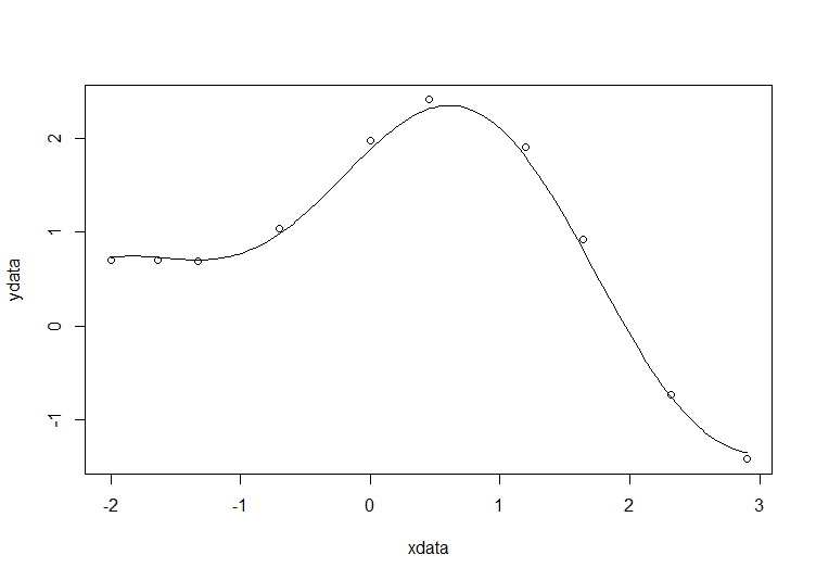
# construct the data vectors using c()
xdata = c(-2,-1.64,-1.33,-0.7,0,0.45,1.2,1.64,2.32,2.9)
ydata = c(0.699369,0.700462,0.695354,1.03905,1.97389,2.41143,1.91091,0.919576,-0.730975,-1.42001)

# look at it
plot(xdata,ydata)

# some starting values
p1 = 1
p2 = 0.2

# do the fit
fit = nls(ydata ~ p1*cos(p2*xdata) + p2*sin(p1*xdata), start=list(p1=p1,p2=p2))

# summarise
summary(fit)

This gives

Formula: ydata ~ p1 * cos(p2 * xdata) + p2 * sin(p1 * xdata)

Parameters:
   Estimate Std. Error t value Pr(>|t|)    
p1 1.881851   0.027430   68.61 2.27e-12 ***
p2 0.700230   0.009153   76.51 9.50e-13 ***
---
Signif. codes:  0 ‘***’ 0.001 ‘**’ 0.01 ‘*’ 0.05 ‘.’ 0.1 ‘ ’ 1

Residual standard error: 0.08202 on 8 degrees of freedom

Number of iterations to convergence: 7 
Achieved convergence tolerance: 2.189e-06

Draw the fit on the plot by getting the prediction from the fit at 200 x-coordinates across the range of xdata

new = data.frame(xdata = seq(min(xdata),max(xdata),len=200))
lines(new$xdata,predict(fit,newdata=new))

Getting the sum of squared residuals is easy enough:

sum(resid(fit)^2)

Which gives

[1] 0.0538127

Finally, lets get the parameter confidence intervals.

confint(fit)

Which gives

Waiting for profiling to be done...
        2.5%     97.5%
p1 1.8206081 1.9442365
p2 0.6794193 0.7209843

9 comments

Simple nonlinear least squares curve fitting in MATLAB

December 6th, 2013

A question I get asked a lot is ‘How can I do nonlinear least squares curve fitting in X?’ where X might be MATLAB, Mathematica or a whole host of alternatives. Since this is such a common query, I thought I’d write up how to do it for a very simple problem in several systems that I’m interested in

This is the MATLAB version. For other versions,see the list below

The problem

xdata = -2,-1.64,-1.33,-0.7,0,0.45,1.2,1.64,2.32,2.9
ydata = 0.699369,0.700462,0.695354,1.03905,1.97389,2.41143,1.91091,0.919576,-0.730975,-1.42001

and you’d like to fit the function

$F(p_1,p_2,x) = p_1 \cos(p_2 x)+p_2 \sin(p_1 x)$

using nonlinear least squares. You’re starting guesses for the parameters are p1=1 and P2=0.2

For now, we are primarily interested in the following results:

The fit parameters
Sum of squared residuals

Future updates of these posts will show how to get other results such as confidence intervals. Let me know what you are most interested in.

How you proceed depends on which toolboxes you have. Contrary to popular belief, you don’t need the Curve Fitting toolbox to do curve fitting…particularly when the fit in question is as basic as this. Out of the 90+ toolboxes sold by The Mathworks, I’ve only been able to look through the subset I have access to so I may have missed some alternative solutions.

Pure MATLAB solution (No toolboxes)

In order to perform nonlinear least squares curve fitting, you need to minimise the squares of the residuals. This means you need a minimisation routine. Basic MATLAB comes with the fminsearch function which is based on the Nelder-Mead simplex method. For this particular problem, it works OK but will not be suitable for more complex fitting problems. Here’s the code

format compact
format long
xdata = [-2,-1.64,-1.33,-0.7,0,0.45,1.2,1.64,2.32,2.9];
ydata = [0.699369,0.700462,0.695354,1.03905,1.97389,2.41143,1.91091,0.919576,-0.730975,-1.42001];

%Function to calculate the sum of residuals for a given p1 and p2
fun = @(p) sum((ydata - (p(1)*cos(p(2)*xdata)+p(2)*sin(p(1)*xdata))).^2);

%starting guess
pguess = [1,0.2];

%optimise
[p,fminres] = fminsearch(fun,pguess)

This gives the following results

p =
1.881831115804464 0.700242006994123
fminres =
0.053812720914713

All we get here are the parameters and the sum of squares of the residuals. If you want more information such as 95% confidence intervals, you’ll have a lot more hand-coding to do. Although fminsearch works fine in this instance, it soon runs out of steam for more complex problems.

MATLAB with optimisation toolbox

With respect to this problem, the optimisation toolbox gives you two main advantages over pure MATLAB. The first is that better optimisation routines are available so more complex problems (such as those with constraints) can be solved and in less time. The second is the provision of the lsqcurvefit function which is specifically designed to solve curve fitting problems. Here’s the code

format long
format compact
xdata = [-2,-1.64,-1.33,-0.7,0,0.45,1.2,1.64,2.32,2.9];
ydata = [0.699369,0.700462,0.695354,1.03905,1.97389,2.41143,1.91091,0.919576,-0.730975,-1.42001];

%Note that we don't have to explicitly calculate residuals
fun = @(p,xdata) p(1)*cos(p(2)*xdata)+p(2)*sin(p(1)*xdata);

%starting guess
pguess = [1,0.2];

[p,fminres] = lsqcurvefit(fun,pguess,xdata,ydata)

This gives the results

p =
   1.881848414551983   0.700229137656802
fminres =
   0.053812696487326

MATLAB with statistics toolbox

There are two interfaces I know of in the stats toolbox and both of them give a lot of information about the fit. The problem set up is the same in both cases

%set up for both fit commands in the stats toolbox
xdata = [-2,-1.64,-1.33,-0.7,0,0.45,1.2,1.64,2.32,2.9];
ydata = [0.699369,0.700462,0.695354,1.03905,1.97389,2.41143,1.91091,0.919576,-0.730975,-1.42001];

fun = @(p,xdata) p(1)*cos(p(2)*xdata)+p(2)*sin(p(1)*xdata);

pguess = [1,0.2];

Method 1 makes use of NonLinearModel.fit

mdl = NonLinearModel.fit(xdata,ydata,fun,pguess)

The returned object is a NonLinearModel object

class(mdl)
ans =
NonLinearModel

which contains all sorts of useful stuff

mdl = 
Nonlinear regression model:
    y ~ p1*cos(p2*xdata) + p2*sin(p1*xdata)

Estimated Coefficients:
          Estimate             SE                 
    p1      1.8818508110535      0.027430139389359
    p2    0.700229815076442    0.00915260662357553

          tStat               pValue              
    p1    68.6052223191956    2.26832562501304e-12
    p2    76.5060538352836    9.49546284187105e-13

Number of observations: 10, Error degrees of freedom: 8
Root Mean Squared Error: 0.082
R-Squared: 0.996,  Adjusted R-Squared 0.995
F-statistic vs. zero model: 1.43e+03, p-value = 6.04e-11

If you don’t need such heavyweight infrastructure, you can make use of the statistic toolbox’s nlinfit function

[p,R,J,CovB,MSE,ErrorModelInfo] = nlinfit(xdata,ydata,fun,pguess);

Along with our parameters (p) this also provides the residuals (R), Jacobian (J), Estimated variance-covariance matrix (CovB), Mean Squared Error (MSE) and a structure containing information about the error model fit (ErrorModelInfo).

Both nlinfit and NonLinearModel.fit use the same minimisation algorithm which is based on Levenberg-Marquardt

MATLAB with Symbolic Toolbox

MATLAB’s symbolic toolbox provides a completely separate computer algebra system called Mupad which can handle nonlinear least squares fitting via its stats::reg function. Here’s how to solve our problem in this environment.

First, you need to start up the mupad application. You can do this by entering

mupad

into MATLAB. Once you are in mupad, the code looks like this

xdata := [-2,-1.64,-1.33,-0.7,0,0.45,1.2,1.64,2.32,2.9]:
ydata := [0.699369,0.700462,0.695354,1.03905,1.97389,2.41143,1.91091,0.919576,-0.730975,-1.42001]:
stats::reg(xdata,ydata,p1*cos(p2*x)+p2*sin(p1*x),[x],[p1,p2],StartingValues=[1,0.2])

The result returned is

[[1.88185085, 0.7002298172], 0.05381269642]

These are our fitted parameters,p1 and p2, along with the sum of squared residuals. The documentation tells us that the optimisation algorithm is Levenberg-Marquardt– this is rather better than the simplex algorithm used by basic MATLAB’s fminsearch.

MATLAB with the NAG Toolbox

The NAG Toolbox for MATLAB is a commercial product offered by the UK based Numerical Algorithms Group. Their main products are their C and Fortran libraries but they also have a comprehensive MATLAB toolbox that contains something like 1500+ functions. My University has a site license for pretty much everything they put out and we make great use of it all. One of the benefits of the NAG toolbox over those offered by The Mathworks is speed. NAG is often (but not always) faster since its based on highly optimized, compiled Fortran. One of the problems with the NAG toolbox is that it is difficult to use compared to Mathworks toolboxes.

In an earlier blog post, I showed how to create wrappers for the NAG toolbox to create an easy to use interface for basic nonlinear curve fitting. Here’s how to solve our problem using those wrappers.

format long
format compact
xdata = [-2,-1.64,-1.33,-0.7,0,0.45,1.2,1.64,2.32,2.9];
ydata = [0.699369,0.700462,0.695354,1.03905,1.97389,2.41143,1.91091,0.919576,-0.730975,-1.42001];

%Note that we don't have to explicitly calculate residuals
fun = @(p,xdata) p(1)*cos(p(2)*xdata)+p(2)*sin(p(1)*xdata);
start = [1,0.2];
[p,fminres]=nag_lsqcurvefit(fun,start,xdata,ydata)

which gives

Warning: nag_opt_lsq_uncon_mod_func_easy (e04fy) returned a warning indicator (5) 
p =
   1.881850904268710   0.700229557886739
fminres =
   0.053812696425390

For convenience, here’s the two files you’ll need to run the above (you’ll also need the NAG Toolbox for MATLAB of course)

MATLAB with curve fitting toolbox

One would expect the curve fitting toolbox to be able to fit such a simple curve and one would be right :)

xdata = [-2,-1.64,-1.33,-0.7,0,0.45,1.2,1.64,2.32,2.9];
ydata = [0.699369,0.700462,0.695354,1.03905,1.97389,2.41143,1.91091,0.919576,-0.730975,-1.42001];

opt = fitoptions('Method','NonlinearLeastSquares',...
               'Startpoint',[1,0.2]);
f = fittype('p1*cos(p2*x)+p2*sin(p1*x)','options',opt);

fitobject = fit(xdata',ydata',f)

Note that, unlike every other Mathworks method shown here, xdata and ydata have to be column vectors. The result looks like this

fitobject = 

     General model:
     fitobject(x) = p1*cos(p2*x)+p2*sin(p1*x)
     Coefficients (with 95% confidence bounds):
       p1 =       1.882  (1.819, 1.945)
       p2 =      0.7002  (0.6791, 0.7213)

fitobject is of type cfit:

 class(fitobject)

ans =
cfit

In this case it contains two fields, p1 and p2, which are the parameters we are looking for

>> fieldnames(fitobject)
ans = 
    'p1'
    'p2'
>> fitobject.p1
ans =
   1.881848414551983
>> fitobject.p2
ans =
    0.700229137656802

For maximum information, call the fit command like this:

[fitobject,gof,output] = fit(xdata',ydata',f)

fitobject = 

     General model:
     fitobject(x) = p1*cos(p2*x)+p2*sin(p1*x)
     Coefficients (with 95% confidence bounds):
       p1 =       1.882  (1.819, 1.945)
       p2 =      0.7002  (0.6791, 0.7213)

gof = 

           sse: 0.053812696487326
       rsquare: 0.995722238905101
           dfe: 8
    adjrsquare: 0.995187518768239
          rmse: 0.082015773244637

output = 

           numobs: 10
         numparam: 2
        residuals: [10x1 double]
         Jacobian: [10x2 double]
         exitflag: 3
    firstorderopt: 3.582047395989108e-05
       iterations: 6
        funcCount: 21
     cgiterations: 0
        algorithm: 'trust-region-reflective'
          message: [1x86 char]

8 comments

Simple nonlinear least squares curve fitting in Maple

December 6th, 2013

A question I get asked a lot is ‘How can I do nonlinear least squares curve fitting in X?’ where X might be MATLAB, Mathematica or a whole host of alternatives. Since this is such a common query, I thought I’d write up how to do it for a very simple problem in several systems that I’m interested in

This is the Maple version. For other versions,see the list below

The problem

xdata = -2,-1.64,-1.33,-0.7,0,0.45,1.2,1.64,2.32,2.9
ydata = 0.699369,0.700462,0.695354,1.03905,1.97389,2.41143,1.91091,0.919576,-0.730975,-1.42001

and you’d like to fit the function

$F(p_1,p_2,x) = p_1 \cos(p_2 x)+p_2 \sin(p_1 x)$

using nonlinear least squares. You’re starting guesses for the parameters are p1=1 and P2=0.2

For now, we are primarily interested in the following results:

The fit parameters
Sum of squared residuals

Future updates of these posts will show how to get other results such as confidence intervals. Let me know what you are most interested in.

Solution in Maple

Maple’s user interface is quite user friendly and it uses non-linear optimization routines from The Numerical Algorithms Group under the hood. Here’s the code to get the parameter values and sum of squares of residuals

with(Statistics):

xdata := Vector([-2, -1.64, -1.33, -.7, 0, .45, 1.2, 1.64, 2.32, 2.9], datatype = float):
ydata := Vector([.699369, .700462, .695354, 1.03905, 1.97389, 2.41143, 1.91091, .919576,  
  -.730975, -1.42001], datatype = float):
NonlinearFit(p1*cos(p2*x)+p2*sin(p1*x), xdata, ydata, x, initialvalues = [p1 = 1, p2 = .2], 
   output = [parametervalues, residualsumofsquares])

which gives the result

[[p1 = 1.88185090465902, p2 = 0.700229557992540], 0.05381269642]

Various other outputs can be specified in the output vector such as:

solutionmodule
degreesoffreedom
leastsquaresfunction
parametervalues
parametervector
residuals
residualmeansquare
residualstandarddeviation
residualsumofsquares.

The meanings of the above are mostly obvious. In those cases where they aren’t, you can look them up in the documentation link below.

Further documentation

The full documentation for Maple’s NonlinearFit command is at http://www.maplesoft.com/support/help/Maple/view.aspx?path=Statistics%2fNonlinearFit

Notes

I used Maple 17.02 on 64bit Windows to run the code in this post.

1 comment

Simple nonlinear least squares curve fitting in Julia

December 6th, 2013

A question I get asked a lot is ‘How can I do nonlinear least squares curve fitting in X?’ where X might be MATLAB, Mathematica or a whole host of alternatives. Since this is such a common query, I thought I’d write up how to do it for a very simple problem in several systems that I’m interested in

This is the Julia version. For other versions,see the list below

The problem

xdata = -2,-1.64,-1.33,-0.7,0,0.45,1.2,1.64,2.32,2.9
ydata = 0.699369,0.700462,0.695354,1.03905,1.97389,2.41143,1.91091,0.919576,-0.730975,-1.42001

and you’d like to fit the function

$F(p_1,p_2,x) = p_1 \cos(p_2 x)+p_2 \sin(p_1 x)$

using nonlinear least squares. You’re starting guesses for the parameters are p1=1 and P2=0.2

For now, we are primarily interested in the following results:

The fit parameters
Sum of squared residuals

Future updates of these posts will show how to get other results such as confidence intervals. Let me know what you are most interested in.

Julia solution using Optim.jl

Optim.jl is a free Julia package that contains a suite of optimisation routines written in pure Julia. If you haven’t done so already, you’ll need to install the Optim package

Pkg.add("Optim")

The solution is almost identical to the example given in the curve fitting demo of the Optim.jl readme file:

using Optim

model(xdata,p) = p[1]*cos(p[2]*xdata)+p[2]*sin(p[1]*xdata)

xdata = [-2,-1.64,-1.33,-0.7,0,0.45,1.2,1.64,2.32,2.9]
ydata = [0.699369,0.700462,0.695354,1.03905,1.97389,2.41143,1.91091,0.919576,-0.730975,-1.42001]

beta, r, J = curve_fit(model, xdata, ydata, [1.0, 0.2])
# beta = best fit parameters
# r = vector of residuals
# J = estimated Jacobian at solution

@printf("Best fit parameters are: %f and %f",beta[1],beta[2])
@printf("The sum of squares of residuals is %f",sum(r.^2.0))

The result is

Best fit parameters are: 1.881851 and 0.700230
@printf("The sum of squares of residuals is %f",sum(r.^2.0))

Notes

I used Julia version 0.2 on 64bit Windows 7 to run the code in this post

1 comment

Simple nonlinear least squares curve fitting in Python

December 6th, 2013

A question I get asked a lot is ‘How can I do nonlinear least squares curve fitting in X?’ where X might be MATLAB, Mathematica or a whole host of alternatives. Since this is such a common query, I thought I’d write up how to do it for a very simple problem in several systems that I’m interested in

This is the Python version. For other versions,see the list below

The problem

xdata = -2,-1.64,-1.33,-0.7,0,0.45,1.2,1.64,2.32,2.9
ydata = 0.699369,0.700462,0.695354,1.03905,1.97389,2.41143,1.91091,0.919576,-0.730975,-1.42001

and you’d like to fit the function

$F(p_1,p_2,x) = p_1 \cos(p_2 x)+p_2 \sin(p_1 x)$

using nonlinear least squares. You’re starting guesses for the parameters are p1=1 and P2=0.2

For now, we are primarily interested in the following results:

The fit parameters
Sum of squared residuals

Future updates of these posts will show how to get other results such as confidence intervals. Let me know what you are most interested in.

Python solution using scipy

Here, I use the curve_fit function from scipy

import numpy as np
from scipy.optimize import curve_fit

xdata = np.array([-2,-1.64,-1.33,-0.7,0,0.45,1.2,1.64,2.32,2.9])
ydata = np.array([0.699369,0.700462,0.695354,1.03905,1.97389,2.41143,1.91091,0.919576,-0.730975,-1.42001])

def func(x, p1,p2):
  return p1*np.cos(p2*x) + p2*np.sin(p1*x)

popt, pcov = curve_fit(func, xdata, ydata,p0=(1.0,0.2))

The variable popt contains the fit parameters

array([ 1.88184732,  0.70022901])

We need to do a little more work to get the sum of squared residuals

p1 = popt[0]
p2 = popt[1]
residuals = ydata - func(xdata,p1,p2)
fres = sum(residuals**2)

which gives

0.053812696547933969

I’ve put this in an Ipython notebook which can be downloaded here. There is also a pdf version of the notebook.

10 comments

Simple nonlinear least squares curve fitting in Mathematica

December 6th, 2013

A question I get asked a lot is ‘How can I do nonlinear least squares curve fitting in X?’ where X might be MATLAB, Mathematica or a whole host of alternatives. Since this is such a common query, I thought I’d write up how to do it for a very simple problem in several systems that I’m interested in

This is the Mathematica version. For other versions,see the list below

The problem

You have the following 10 data points

xdata = -2,-1.64,-1.33,-0.7,0,0.45,1.2,1.64,2.32,2.9
ydata = 0.699369,0.700462,0.695354,1.03905,1.97389,2.41143,1.91091,0.919576,-0.730975,-1.42001

and you’d like to fit the function

$F(p_1,p_2,x) = p_1 \cos(p_2 x)+p_2 \sin(p_1 x)$

using nonlinear least squares. You’re starting guesses for the parameters are p1=1 and P2=0.2

For now, we are primarily interested in the following results:

The fit parameters
Sum of squared residuals

Future updates of these posts will show how to get other results such as confidence intervals. Let me know what you are most interested in.

Mathematica Solution using FindFit
FindFit is the basic nonlinear curve fitting routine in Mathematica

xdata={-2,-1.64,-1.33,-0.7,0,0.45,1.2,1.64,2.32,2.9};
ydata={0.699369,0.700462,0.695354,1.03905,1.97389,2.41143,1.91091,0.919576,-0.730975,-1.42001};

(*Mathematica likes to have the data in the form {{x1,y1},{x2,y2},..}*)
data = Partition[Riffle[xdata, ydata], 2];

FindFit[data, p1*Cos[p2 x] + p2*Sin[p1 x], {{p1, 1}, {p2, 0.2}}, x]

Out[4]:={p1->1.88185,p2->0.70023}

Mathematica Solution using NonlinearModelFit
You can get a lot more information about the fit using the NonLinearModelFit function

(*Set up data as before*)
xdata={-2,-1.64,-1.33,-0.7,0,0.45,1.2,1.64,2.32,2.9};
ydata={0.699369,0.700462,0.695354,1.03905,1.97389,2.41143,1.91091,0.919576,-0.730975,-1.42001};
data = Partition[Riffle[xdata, ydata], 2];

(*Create the NonLinearModel object*)
nlm = NonlinearModelFit[data, p1*Cos[p2 x] + p2*Sin[p1 x], {{p1, 1}, {p2, 0.2}}, x];

The NonLinearModel object contains many properties that may be useful to us. Here’s how to list them all

nlm["Properties"]

Out[10]= {"AdjustedRSquared", "AIC", "AICc", "ANOVATable", \
"ANOVATableDegreesOfFreedom", "ANOVATableEntries", "ANOVATableMeanSquares", \
"ANOVATableSumsOfSquares", "BestFit", "BestFitParameters", "BIC", \
"CorrelationMatrix", "CovarianceMatrix", "CurvatureConfidenceRegion", "Data", \
"EstimatedVariance", "FitCurvatureTable", "FitCurvatureTableEntries", \
"FitResiduals", "Function", "HatDiagonal", "MaxIntrinsicCurvature", \
"MaxParameterEffectsCurvature", "MeanPredictionBands", \
"MeanPredictionConfidenceIntervals", "MeanPredictionConfidenceIntervalTable", \
"MeanPredictionConfidenceIntervalTableEntries", "MeanPredictionErrors", \
"ParameterBias", "ParameterConfidenceIntervals", \
"ParameterConfidenceIntervalTable", \
"ParameterConfidenceIntervalTableEntries", "ParameterConfidenceRegion", \
"ParameterErrors", "ParameterPValues", "ParameterTable", \
"ParameterTableEntries", "ParameterTStatistics", "PredictedResponse", \
"Properties", "Response", "RSquared", "SingleDeletionVariances", \
"SinglePredictionBands", "SinglePredictionConfidenceIntervals", \
"SinglePredictionConfidenceIntervalTable", \
"SinglePredictionConfidenceIntervalTableEntries", "SinglePredictionErrors", \
"StandardizedResiduals", "StudentizedResiduals"}

Let’s extract the fit parameters, 95% confidence levels and residuals

{params, confidenceInt, res} = 
 nlm[{"BestFitParameters", "ParameterConfidenceIntervals", "FitResiduals"}]

Out[22]= {{p1 -> 1.88185, 
  p2 -> 0.70023}, {{1.8186, 1.9451}, {0.679124, 
   0.721336}}, {-0.0276906, -0.0322944, -0.0102488, 0.0566244, 
  0.0920392, 0.0976307, 0.114035, 0.109334, 0.0287154, -0.0700442}}

The parameters are given as replacement rules. Here, we convert them to pure numbers

{p1, p2} = {p1, p2} /. params

Out[38]= {1.88185,0.70023}

Although only a few decimal places are shown, p1 and p2 are stored in full double precision. You can see this by converting to InputForm

InputForm[{p1, p2}]

Out[43]//InputForm=
{1.8818508498053645, 0.7002298171759191}

Similarly, let’s look at the 95% confidence interval, extracted earlier, in full precision

confidenceInt // InputForm

Out[44]//InputForm=
{{1.8185969887307214, 1.9451047108800077}, 
 {0.6791239458086734, 0.7213356885431649}}

Calculate the sum of squared residuals

resnorm = Total[res^2]

Out[45]= 0.0538127

Notes
I used Mathematica 9 on Windows 7 64bit to perform these calculations

4 comments

Archive for December, 2013

Computing Eigenvalues without balancing in Python using the NAG library

Christmas cards from Mathematical Software

Simple nonlinear least squares curve fitting in R

Simple nonlinear least squares curve fitting in MATLAB

Simple nonlinear least squares curve fitting in Maple

Simple nonlinear least squares curve fitting in Julia

Simple nonlinear least squares curve fitting in Python

Simple nonlinear least squares curve fitting in Mathematica

Categories

Archives

Blogroll

Meta

Archive for December, 2013

Share this:

Share this:

Share this:

Share this:

Share this:

Share this:

Share this:

Share this:

Categories

Archives

Blogroll

Meta