
Archive for December, 2008
Those of you who know me personally will know that it takes a lot to stun me into silence but the story in the following link did just that. I’d say more about it but am too stunned for words….
http://linuxlock.blogspot.com/2008/12/linux-stop-holding-our-kids-back.html
Mathematica 7 includes some very nice support for parallel computing and one of the easiest commands to use is Parallelize. If you have a multi-core computer (and most of them are these days) then, in some cases, you can get a speedup of a factor of 2 or more simply by wrapping your code with the Parallelize command. I’ll stress that it’s not always this easy but, when it is, it’s very nice.
To start getting my head around the new command I looked at the following small piece of code which is included in the Mathematica 7 documentation.
data = Table[ PrimeQ[n! + 1], {n, 400, 550}];
This code calculates numbers of the form n!+1 for n between 400 and 550 and tests to see if they are prime or not. Let’s see how long it takes on my dual core 2Ghz Dell XPS M1330:
data = Table[ PrimeQ[n! + 1], {n, 400, 550}]; // AbsoluteTiming
Out[1]={14.092809, Null}
We see from the above that it took just over 14 seconds before we apply any parallelism. Let’s see how much improvement we get by using the Parallelize command:
data = Parallelize[Table[ PrimeQ[n! + 1], {n, 400, 550}]]; // AbsoluteTiming

Out[2]= {21.124572, Null}
Oh dear, something has gone drastically wrong! The parallel calculation is taking 7 seconds (or 50%) longer than the serial calculation. Before writing a bug report to Wolfram, I thought I would dig around a little to try and work out what was going on.
First things first, let’s take a look at how hard Mathematica is pushing the processor in both cases. I can add a little CPU monitoring applet to my GNOME panel by right clicking on it and selecting add to Panel. From the resulting list I choose CPU Frequency Scaling Monitor.
When I initially did this, the applet informed me that my CPU was running at 800 Mhz – way below its maximum speed of 2Ghz. When I click on this applet I get a range of settings that could be applied to my CPU such as On demand, Performance and Powersave along with specific speed settings from 800Mhz to 2 Ghz. The one selected was on demand.
Turning back to Mathematica I run the sequential code again
data = Table[ PrimeQ[n! + 1], {n, 400, 550}]; // AbsoluteTiming

Out[3]={14.117028, Null}
According to the CPU Monitor, my computer was running at 2Ghz (its top speed) during the entire calculation. However, when I ran the Parallelize version, the processor speed remained at 800Mhz the whole time. So, the calculation may well have been running in parallel but each of the 2 cores was only running at 40% of top speed. The problem seems to lie with Mathematica’s interaction with the on demand setting of the processor manager.
By clicking on the GNOME CPU monitor, I can fix the processor to run at 2Ghz at all times – no fancy processor management here – just the fastest speed my computer can manage. Let’s see what the results of the two versions of the code are when I do this.
data = Table[ PrimeQ[n! + 1], {n, 400, 550}]; // AbsoluteTiming
Out[4]={14.062377, Null}
data = Parallelize[Table[ PrimeQ[n! + 1], {n, 400, 550}]]; // AbsoluteTiming
Out[5]={7.635570, Null}
That’s more like it! The parallel version is almost twice as fast as the serial version – just as we would expect on a dual core system. So, the moral of the story is to ensure that you don’t have your system set to modify it’s processor speed on demand when trying to make use of the new Parallel features of Mathematica 7.
For the record I am running GNOME 2.24.1 on Ubuntu 8.10 with Mathematica 7.
Since setting the Walking Randomly Christmas Challenge, I have been looking around the web for Christmasy things that other people have written using mathematical software. If you have been thinking of submitting something to the challenge then maybe these will give you inspiration.
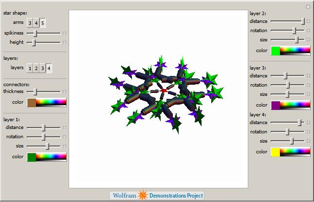
First up, we have several Wolfram Demonstrations based on themes that could be used to design Christmas greeting cards. For example there is a great one by Michael Trott and Jeff Bryant called Decorative Holiday Stars.
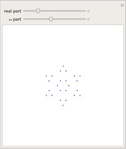
If you prefer your greetings less ‘designer’ and more purely Mathematical then how about creating a card from Eisenstein Snowflakes?
Other Wolfram Demonstrations that might give you inspiration for the Christmas challenge include
I next turned my attention to MATLAB and their File Exchange and immediately hit upon a MATLAB file by Marc Lätzel that draws a Christmas tree.

Something a bit more mathematical is the .m file by Per Sundqvist which generates a FEMLAB geometry for the Koch snowflake. This can then be used in FEMLAB to solve eigenvalue problems over the Koch domain. I don’t have a copy of FEMLAB (called COMSOL these days) so I can’t test it but the result looks nice and a quick google search has resulted in some references that might be useful in implementing calculations like this. ‘Computing eigenfunctions on the Koch Snowflake: a new grid and symmetry‘ by John M Neuberger might be a good place to start.

Next up is Maple. A quick search of their Application Centre resulted in the Maple 5 code for a swinging snowman – very nice! This is another one I can’t test because, unfortunately, I don’t have a copy of Maple but if you are one of those who do then the source code is available if you’d like to try it out. Maple is at version 12 these days so it will be interesting to see if this old Maple 5 code still runs (let me know if you are able to test it).

These above examples are just highlights of the sort of thing I discovered while looking around for ‘Christmas maths.’ Why not try your hand at designing something yourself in the Walking Randomly Christmas Challenge? Submissions can be in pretty much any language you care to mention although, of the commercial maths packages, I can only test scripts written in Mathematica, Mupad, MATLAB and MathCAD. Of course any open-source package (such as SAGE or Octave) is fair game.
If you prefer your submission to be anonymous then either don’t let me know who you are (post your code in the comments section for example) or just tell me that you would prefer it if your name were not attached. Of course if you want full recognition for your talents then I can do that too :) My email address is relatively easy to find. Have fun!
Almost 10 years ago now, I was a teaching assistant for an Introduction to Fortran course at the University of Sheffield. I remember being told by one of the other PhD students that ‘Fortran is a dying language and so we are wasting our time teaching this stuff. No one will be using Fortran in 10 years time.’
Fast forward 10 years and Fortran is still going strong in the research and numerical communities. If you are doing numerics and you want fast code then Fortran is an option that you simply can’t ignore. It is also required for doing things like writing user defined materials in the finite element analysis package, Abaqus. One of the best Fortran compilers on the market (in my opinion at least) is the NAG Fortran Compiler and their Linux version has recently been updated to version 5.2.
It now includes support for almost all of the features in the Fortran 2003 standard and they have also added quadruple precision support – something that the people I support have wanted for a long time. A full list of changes can be found on NAG’s website.
Finally a note to self – they have changed the name of the executable from f95 to nagfor – this will generate support queries…you know it will!
I have no idea where the following joke originated but you can find it all over the web. At least one person disagrees with the calculations ;)
1. No known species of reindeer can fly, but there are 300,000 species of living organisms yet to be classified, and while most of these are insects and germs, this does not completely rule out flying reindeer which only Santa has seen.
2. There are 2 billion children in the world (persons under 18). But since Santa doesn’t (appear) to handle Muslim, Hindu, Jewish, or Buddhist children, that reduces the workload by 85% of the total, leaving 378 million according to the Population Reference Bureau. At an average (census) rate of 3.5 children per household, that’s 91.8 million homes. One presumes there is at least one good child per house.
3. Santa has 31 hours of Christmas to work with, thanks to the different time zones and the rotation of the earth, assuming he travels east to west (which seems logical). This works out to 822.6 visits per second. This is to say that for each Christian household with good children, Santa has 1/1000th of a second to park, hop out of the sleigh, jump down the chimney, fill the stocking, distribute the remaining presents under the tree, eat whatever snacks have been left, get back up the chimney, get back into the sleigh and move on to the next house. Asusming that each of these 91.8 million stops are evenly distributed around the earth, which, of course, we know to be false, but for the purposes of our calculations we will accept, we are now talking about 0.78 miles per household, for a total trip of 75.5 million miles, not counting stops to do what most of us do at least once every 31 hours, plus feeding, etc. That means that Santa’s sleigh is moving at 650 miles per second, 3000 times the speed of sound. For purposes of comparison, the fastest man-made vehicle on earth, the Ulysses space probe, moves at a poky 27.4 miles per second – a conventional reindeer can run, at tops 15 miles per hour.
4. The payload on the sleigh adds another interesting element. Assuming each child gets nothing more than a medium sized lego set (2 pounds), the sleigh is carrying 321,300 tons, not counting Santa, who is invariably described as overweight. On land, conventional reindeer can pull no more than 300 pounds. Even granting the “flying reindeer” can pull TEN TIMES the normal amount, we cannot do the job with eight, or even nine. We need 214,200 reindeer. This increased the payload – not even counting the weight of the sleigh to 353,430 tons. Again, for comparison – this is four times the weight of the Queen Elizabeth – 5,353,000 tons travelling at 650 miles per second creates enormous air resistance. This will heat the reindeer up in the same fashion as spacecrafts re-entering the earth’s atmosphere. The lead pair will absorb 14.3 quintillion joules of energy per second each. In short, they will burst into flames almost instantaneously, exposing the reindeer behind them, and creating a deafening sonic boom in their wake. The entire reindeer team will be vaporized with 4.26 thousandths of a second. Santa, meanwhile, will be subject to centrifugal forces 17,500.06 times greater than gravity. A 250 pound Santa (which seems ludicrously slim) would be pinned to the back of the sleigh by a 4,315,015 pound force.