
Archive for the ‘mathematica’ Category
A few years ago, while working through a degree in theoretical physics at Sheffield University, I took a course on special functions in physics that was given by the legendary lecturer Dr Stoddart (saviour of many a physics undergraduate, including me, during his many years there – please leave a comment if you studied at Sheffield and remember him).
This course introduced me to the fascinating world of the so called ‘higher transcendental functions’ of mathematical physics. I remember that we covered topics such as Bessel functions, Laguerre polynomials, Hermite Polynomials and the Gamma function among others but in a one semester course we only really scratched the surface of the subject.
Since then I have come across several other special functions during the course of my work such as the LambertW function, Mathieu functions, Chebyshev polynomials and more. I used to be a physicist and so, despite the fact that the theory behind these functions can often be fascinating, all I had time to consider back then was how to evaluate them.
In fact, as far as my professional life goes, the question of evaluation is still the only thing that I get asked about regarding special functions. Questions such as ‘How can I evaluate the LambertW function in MATLAB?’ (Answer – by using this user-defined function) or ‘Do you know of a free, open source, implementation of Bessel’s function?’ (Answer – the GNU Scientific Library).
The idea for this post came to me while reading an article written in 1994 (and subsequently updated in 2000) where the authors discussed the Numerical Evaluation of Special Functions. One of the features of this document was a list of various special functions combined with a list of software packages that could evaluate them. For example it lists Dawson’s integral and tells us that if you need to evaluate this then you can use various software packages such as the NAG libraries or Numerical Recipes.
I thought that this was a very useful document but a major problem with it is that it is rather out of date! Wouldn’t it be great if someone were to create an updated version that included all of the latest advances in software libraries and applications. I even idly thought of attempting to do this myself and publish the results here but it turns out that I have (thankfully) been beaten to it.
It’s not finished yet but the NIST Digital Library of Mathematical Functions looks like it is going to be exactly what I need. Apparently this project aims to be a sort of modern rewrite of Abramowitz and Stegun’s Handbook of Mathematical Functions, a book that almost every physicist I knew had a copy of. The preview looks very promising to say the least! For example, take the section on the Gamma Function. The library contains everything you might want to know about this function such as its definition, 2D and 3D plots of its graphs, its series expansion and, of course, a list of software packages and libraries that can be used to evaluate it. I note that, for the Gamma function, one can choose from MATLAB, Mathematica, MAPLE, NAG, Maxima, PARI-GP, the GSL, Numerical Recipes and several others – not exactly short of Gamma function implementations are we?
When it’s finished, the work will be published as a book called ‘Handbook of Mathematical Functions’ but will also be available freely online as a digital library – fabulous!
Some time ago now I worked with Will Robertson to produce a package that allowed Mathematica users to add MATLAB like colorbars to their graphs. The package was called ColorbarPlot and version 0.3 was released on Wolfram’s Library Archive last October. It was very well received and we were both pleased to find that people were actually finding it useful. The feature requests started rolling in and Will and I started to hack in extra bits of functionality as they were requested. Eventually, we had enough new features hacked in to demand a rewrite which Will duly did and the resulting version 0.4 of the ColorbarPlot package was sent out to a few users a little while ago.
We refrained from actually announcing it though since we wanted this new version to replace the old one in the Wolfram Library. Will sent them an email ages ago but has heard nothing and so we decided to just publish it ourselves. So, without further ado, here is a link to a zip file containing the ColorbarPlot package itself along with an examples notebook.
Think of this as a ‘snapshot’ of the live package – it will never change and is hosted on my server. If you have googled your way here and are wondering if there is a newer version then you should take a look at Will’s GitHub repository where you will always be able to find the latest version of ColorbarPlot along with some other packages that he has authored. Will’s own announcement of this upgrade can be found on his website.
So, what’s new in this version? The most useful change is that you can now add colorbars to List based plots – useful for experimental data. The following piece of Mathematica code creates a List of data and uses ColorbarPlot to plot it.
data2d = Table[Sin[x y^2], {x, -2, 2, 0.1}, {y, -2, 2, 0.1}];
ColorbarPlot[data2d, PlotType -> “Contour”]

Of course you are not limited to just 2D list based plots
ColorbarPlot[data2d, PlotType -> “3D”]
ColorbarPlot[data2d, PlotType -> “Point3D”]

The full list of Plot types you can use with ColorbarPlot is
- (List)ContourPlot
- (List)DensityPlot
- (List)Plot3D
- ListPointPlot3D
Other new features include the ability to manually choose the min/max scale of the colorbar, the ability to fine tune the padding and height of the colorbar along with various clean ups and bug fixes. All new (and old) features are documented and demonstrated in the accompanying examples notebook. Thanks to Will for his hard work on this release (he did most of it – my contributions are rather small this time).
Feedback and suggestions are, as always, very welcome. If you publish any results using this package then please let me know – it would be great to see.
Although Mathematica 6 has been out for quite a while now there are still some people at my university who refuse to upgrade from Mathematica 5.2 for one reason or another. Some don’t like the new help system, others don’t have the time to rewrite teaching notes and some find that their old Mathematica scripts simply don’t run properly in version 6 and they can’t figure out why.
Of course most users have embraced the new version as there is simply too much new functionality to do otherwise. Some people, however, have minor problems with version 6 that might not be show stoppers but are definitely annoying. One such problem was reported to me today by a user who was missing the “Evaluate Notebook” option that used to be present in the menu of version 5.2.
Fortunately things like this are easily fixed. Within a standard Mathematica install, there is a file called MenuSetup.tr which defines what appears on the menus. On my Windows system it appears in the following location
C:\Program Files\Wolfram Research\Mathematica\6.0\SystemFiles\FrontEnd\TextResources\Windows\MenuSetup.tr
To get “Evaluate Notebook” to appear in the “Evaluation” part of the menu just modify this file by adding the line
Item[“Evaluate &Notebook”, “EvaluateNotebook”],
after the part that reads
Menu[“E&valuation”,
{
Let me know if you find this useful.
I recently upgraded my Ubuntu installation from 7.10 to 8.04 and almost immediately ran into problems when trying to run Mathematica 6.0.2 – all of the fonts are not rendering properly. In addition, if I run mathematica from a console window I get error messages like
X Error of failed request: RenderBadPicture (invalid Picture parameter)
Major opcode of failed request: 158 (RENDER)
Minor opcode of failed request: 7 (RenderFreePicture)
Picture id in failed request: 0x440189f
Serial number of failed request: 69419
Current serial number in output stream: 69420
X Error of failed request: BadMatch (invalid parameter attributes)
Major opcode of failed request: 158 (RENDER)
Minor opcode of failed request: 4 (RenderCreatePicture)
Serial number of failed request: 71071
Current serial number in output stream: 71074
The following screenshot shows the problem – you cannot see anything you type apart from a few symbols such as [] and {} .

Other people have come across this problem and workarounds have been identified. The first is to run Mathematica from a console prompt as follows
mathematica -defaultvisual
This allows you to see what you are doing but is a big ugly. Another workaround is to install libqt4-core and libqt4-gui by doing
sudo apt-get install libqt4-core libqt4-gui
and then rename a couple of files in the Mathematica distribution as follows
sudo mv /usr/local/Wolfram/Mathematica/6.0/SystemFiles/Libraries/Linux/libQtCore.so.4 /usr/local/Wolfram/Mathematica/6.0/SystemFiles/Libraries/Linux/libQtCore.so.4.old
sudo mv /usr/local/Wolfram/Mathematica/6.0/SystemFiles/Libraries/Linux/libQtGui.so.4 /usr/local/Wolfram/Mathematica/6.0/SystemFiles/Libraries/Linux/libQtGui.so.4.old
This fixes the problem but you may get two extra blank windows appear when you run Mathematica. To fix this open up the Option Inspector in Mathematica as follows:
Edit-> Preferences and click on Open Option Inspector
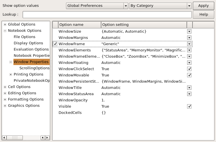
When in the Option Inspector click on Notebook Options and then Window Properties and change the WindowFrame option from “Normal” to “Generic” then click on Apply
A big thank you to the people in this thread on launchpad.net for developing all of these workarounds. I will be reporting these problems to Wolfram’s tech support as soon as I have finished writing this.
Update: 28 May 2008
Someone from Wolfram responded to these issues in this thread. For anyone who has googled themselves here I have copied and pasted his response below:
Note – this is not an “official” Wolfram response, I just wanted to let you all know we’re aware of the issues…
With that in mind, a few comments:
The original error messages are due to X11 providing an incorrect visual buffer to draw on – the ‘export XLIB_SKIP_
The extra windows are supposed to be hidden, and will go back into hiding with 6.0.3 (coming very soon).
The font rendering issues are related to Hardy’s lack of some fonts we normally assume to be installed by default, namely a decent Courier and Times fonts. Some adjustments were made for 6.0.3, but if these do not resolve your issues, you may want to adjust the substitution rules (Option Inspector->Global Options->Menu Settings-
On deleting/replacing libQt* – this is not recommended, as we ship a commercial version of the Qt library, which can potentially differ from the open source version. If it works for now, that’s fortunate, but I would not consider that a permanent fix. We will be updating our shipping version of Qt with our next major release, most likely from the Qt 4 .3 version tree, as 4.4 is causing some compatibility issues (the above mentioned QObject warnings)
I will be attending the 9th International Mathematica Symposium (IMS) next month in Maastricht and wondered if any readers of this blog would be there. Feel free to let me know in the comments if you are and would like to meet up. If you don’t want your comment published just say so and I will withold it after getting your email address.
The minimization of the Rosenbrock function is a classic test problem that is extensively used to test the performance of different numerical optimization algorithms. It was first introduced in 1960 by H.H Rosenbrock in his paper, “An Automatic Method for Finding the Greatest or Least Value of a Function, Computer J. 3, 175-184, 1960 (See here for Rosenbrock’s account of how he came to write that paper.)
The function definition is given below and, although it looks harmless enough, it turns out to be quite challenging to find it’s minimum point by numerical methods.

Acording to Google Scholar, Rosenbrock’s paper has been cited no less than 596 times (as of April 9th 2008) and the function he introduced has been used as a test problem for many different numerical solvers including those in the Matlab Optimization toolbox, The NAG libraries, COMSOL and SciPy (A python module).
So why is this innocuous looking function so difficult to minimise? To answer that let’s first take a look at its contour plot using Mathematica.
ContourPlot[(1 – x)^2 + 100 (y – x^2)^2, {x, -2, 2}, {y, -2, 2},
ContourShading -> False, Contours -> Table[10^-i, {i, -2, 10, 0.5}]
, Epilog -> {Black, PointSize[Large], Point[{1, 1}]}]
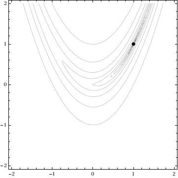
The global minimum of the Rosenbrock function lies at the point x=1, y=1 and is shown in the above diagram by a black spot. Note that the contours are not evenly spaced in this diagram – they are logarithmically spaced instead so the solution lies inside a very deep, narrow, banana shaped valley. The distinctive shape of this function’s contour lines is the reason for its alternative name – “Rosenbrock’s banana function”.
The valley causes a lot of problems for search algorithms such as the method of steepest descents which will quickly find the ‘entrance’ to the valley and then spend hundreds of iterations zigzagging from one side of it to the other – making very slow progress towards the minimum itself.
There is a Mathematica function called FindMinimum that can handle this kind of optimization problem and I wondered how its methods would handle the Rosenbrock function. In the back of my mind I thought that I might also be able to make a nice Wolfram Demonstration from the investigation. While looking at the documentation for FindMinimum I found an example that pretty much solved the problem for me.
pts = Reap[FindMinimum[(1 – x)^2 + 100 (-x^2 – y)^2, {{x, -1.2}, {y, 1}}, StepMonitor :> Sow[{x, y}]]][[2, 1]];
pts = Join[{{-1.2, 1}}, pts];
This finds the minimum point from a starting point of x=-1.2, y=1 and also stores all of the intermediate steps so you can see the path that Mathematica takes in looking for the solution. The only other piece of information needed was to find out how to specify the solution method. It turns out that this is obvious – just use the option
Method->”MethodNameHere”
replacing MethodNameHere with whatever method you want Mathematica to use. You can choose from ConjugateGradient, LevenbergMarquardt, Newton, QuasiNewton, PrincipalAxis and InteriorPoint.
All that remained was to wrap this up in a Manipulate statement, make it look pretty, add some controls and submit it to the demonstrations project. The result can be found here.
One of the things I like about the process of submitting demonstrations to the project is that they are refereed. Someone will take the time to look at your code and make suggestions and small modifications before it gets published. This reduces the possibility of mistakes being made in the final version and really helps with the learning process. Almost every time I have submitted something, I have learned a little more about Mathematica – and that’s really the main reason for me doing it (well its also fun to have your name “up in lights” if I am being honest).
At this point I would like to thank the members of the Wolfram Demonstrations team who have dealt with my submissions so far – not only have they been a pleasure to work with and extremely patient but they have also spared my blushes by pointing out some very stupid mistakes in my code. Of course any that remain are my fault and not theirs.
Just a quick one – someone sent me the following Mathcad bug report and so I thought I would share it. No problems with it in Mathematica or Matlab (using the symbolic toolbox). I find symbolic integration bugs interesting – especially if they come from one of the well known commercial packages such as Mathematica, Maple, Matlab or Mathcad. If you ever come across any then please do let me know in the comments.
The correct answer is Pi/8- 1/Pi which evaluates to about 0.074 so you can see from the image below that Mathcad gets the correct numerical result but fails to get the symbolic result.

In a recent post I asked if anyone had any requests for any Wolfram Demonstrations that they would like to see made. Maria Andersen of the Teaching College Math Technology Blog requested a demonstration that would produce music from the decimal expansion of rational numbers in the same way that this one does for irrational numbers. Well, I always aim to please so here it is:
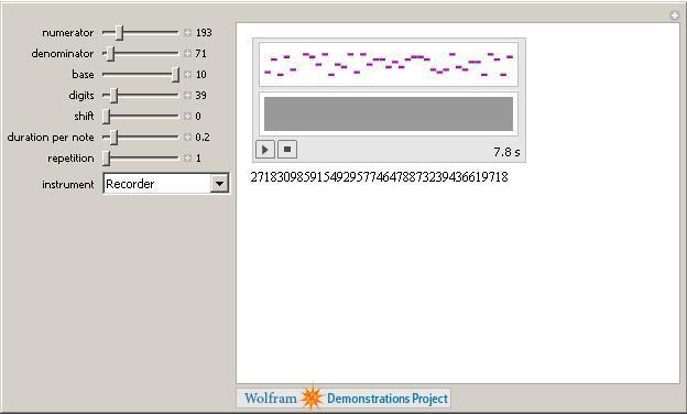
Just set the numerator and denominator with the sliders, choose the base of the result, the number of digits etc, along with what instrument you want and then click play. Remember, if you don’t have Mathematica then you can always use their free MathPlayer to run this demonstration. I hope this is what you were looking for Maria but if it isn’t then let me know what you would like changed and I will see what I can do.
If anyone else has any Wolfram Demonstration requests then leave a comment and I might just code it up for you (unless someone beats me to it of course).
1.Take one dare from Kathryn Cramer and obtain a picture from her website.
2. Steal ideas from this demonstration by Jeff Bryant.
3. Type the following incantations into Mathematica
SetDirectory[“/home/mike/Desktop/random”];
image = Import[“kramer.jpg”];
xpos[x_] := Floor[x/N[2/374.] + 377/2.]
ypos[x_] := Floor[x/N[2/499.] + 502/2.]
imcol[x_, y_] := image[[1]][[1]][[xpos[x]]][[ypos[y]]]/256.;
a = 1; b = 0.9; c = 1;
Plot3D[{Sqrt[ c^2*(1 – (x^2/a^2 + y^2/b^2))], -Sqrt[c^2*(1 – (x^2/a^2 + y^2/b^2))]}, {x, -1, 1}, {y, -1, 1}, ColorFunction -> (RGBColor[imcol[#1, #2]] &), Boxed -> False, Axes -> False, AspectRatio -> 2, ViewAngle -> Pi/13, ViewPoint -> {-3.00336, 0.86708, 3.14159}, PlotRange -> All, Mesh -> False, PlotPoints -> 400]
Enjoy!

I have been playing with the new release of Mathematica for a little while now and thought that I would share what I have found. Now, as indicated by the small increment in version number, this is a minor release and so we should not be expecting anything earth shattering. The sort of things that one expects in a minor release like this include things such as bug-fixes, small performance enhancements, documentation upgrades etc. So…let’s see what he have got.
First on the list are some changes to the documentation center. Copying and pasting from Wolfram’s press release:
- New Virtual Book documentation with updated Mathematica Book content
- New Function Navigator, an easily browsable overview of all Mathematica objects
Let’s start with the Virtual book – what’s that all about? Like Gavin Scott, the writer of this forum message, I went to the help browser and searched for ‘virtual book’ hoping to be enlightened. Nothing – not a single search result! I found this surprising since Wolfram Research felt that it was such an important modification that they chose it to be the first thing they mentioned on their press release. To be honest I probably would not have noticed the new virtual book icon in the help browser without Gavin’s help. To help you find it I have circled it in red in the image below

Clicking on this icon opens the virtual book itself (see the image below) which is essentially an alternative way to navigate the documentation system. This might not seem like much to the casual observer but since the release of version 6 many people have been complaining about the changes made in the documentation system since version 5.2. The Virtual Book is Wolfram’s attempt at addressing some of these complaints by adding some structure that is reminiscent of the original Mathematica Book and I don’t think its too bad at all.
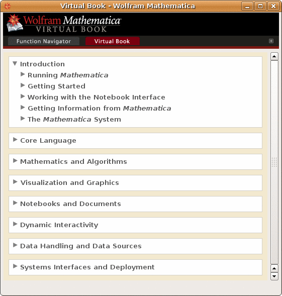
Personally, I have gotten used to the new Documentation center and, although I feel it has some problems, I quite like it – especially the huge number of examples that it contains. However, it does contain a massive quantity of information which is sometimes difficult to navigate through so the extra layer of structure that the Virtual Book provides is a welcome addition.
Next up we have the Function Navigator (below) which, like the Virtual Book, is yet another way to navigate through the documentation. Now this is something that I feel will be very useful – particularly when you are exploring a new area of functionality in Mathematica.
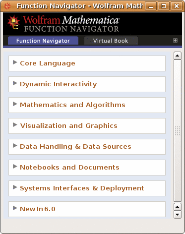
Say that you need to do some statistical calculations and you want to see what functions are available to you in Mathematica. Start off by expanding Mathematics and Algorithms followed by statistics to reveal the window below.

Clicking on our area of interest (Random Number Generation say) will reveal all of the functions available in that area. This is a very useful addition to the help system in my opinion. One minor issue with both the Virtual Book and the Function Navigator is that the windows take longer than expected to initialize. I conducted all of my tests on a pretty fast dual core machine with 4gb RAM and it took almost 3 seconds for the window to appear from the instant I clicked on the icon. I imagine that it is going to be painfully slow on my laptop which has a much lower specification but I haven’t tested it yet. At least one other person has noticed this issue.
The next item on Wolfram’s press release is
- Several additional documentation enhancements, including performance improvements, indexing, and link trails
I simply cannot comment on this as they have not given any examples and I cannot see any obvious changes. Would anyone care to enlighten me? Moving on…
- Full 64-bit performance on Intel Macs
This is great news if you are an owner of an Intel Mac but I’m not so onto the next item.
That’s great but it would be even better if Wolfram were more specific on this. There are some extra details on Wolframs blog post concerning 6.0.2 but even that doesn’t tell the full story. Quoting from Wolfram’s blog:
“A few examples are dramatic compression of graphics that include transparency exported to PDF, more robust embedding of graphics in TeX, and full support for all metadata in FITS images.”
What I would have really liked to have seen here is a comprehensive list of the improvements made – not just a select few. The next few points on Wolfram’s list are all related to the above
- Significant speedup in import of binary data files
- Improved handling of graphics when exporting to TeX and PDF
- Enhanced import of metadata from FITS astronomical image files
The final point Wolfram makes about this new release is
- New coordinate-picking tool and improved highlighting of graphical selections for interactive graphics
This is discussed in detail in the Wolfram’s blog so I will leave it to them to explain what this new feature is. In short – it’s fantastic! I may blog about it myself soon as it looks like it might be extremely useful.
That pretty much covers everything that Wolfram has released concerning this update and apart from the changes in the documentation (which are welcome improvements) it all seems a bit vague to me. I am the administrator for a large university site license and already I have people asking me if the upgrade is worth it if you are coming from version 6.0.1. My current response is along the lines of “well for us its essentially free (more accurately we have paid for it in advance) so you may as well” but if I had to pay extra for it then I probably wouldn’t bother.
The reason that I wouldn’t bother to pay for an upgrade is not because I think it is a bad product – quite the opposite in fact as it is a superb product – but if one is happily using version 6.0 or 6.0.1 then Wolfram Research simply haven’t given us the information we need to decide if we should upgrade or not.
With a bit of googling I eventually came up with some more details that I wished Wolfram would have released publicly. All of the following have been gleaned from posts to newsgroups.
csv files – original source -> here
There is a subtle change in the way .csv files are imported at 6.02.
Put the following into a .csv file:
“hope”
1
2
At 6.01 (and earlier versions of Mathematica) the string was read in as
“hope”. At 6.02 the quotes are included in the string – “\”hope\””.
Integration bug fix – original source -> here
N[Integrate[Log[z] Log[1 + Sqrt[1 – z^2]], {z, 0, 1}]] = -0.707202 (version 6 – incorrect)
N[Integrate[Log[z] Log[1 + Sqrt[1 – z^2]], {z, 0, 1}]] = -0.659589 (version 6.0.2 – correct)
Various improvements – original source -> here
- Fix for a big slowdown in FactorInteger
- Fixes for some wrong Integrate results pointed out by external users
- A few Series fixes
- A few Simplify/FullSimplify/FunctionExpand fixes
- Faster and more reliable numericizing of MeijerG
- A few fixes in special function evaluation
- Fix for RamanujanTau with large arguments
That’s the sort of thing I want to see – details.
I want to see a big list of bug fixes so that I can point to them and say to a user “the new version fixes all of these – if they affect you then you need to upgrade”
I want to see a list of performance enhancements so that I can point to them and say to a user “the new version is faster in all of these areas – if you need them then you need to upgrade”
I want to see a list of changes in function behaviour (such as the csv example above) so that I can explain to someone why their 6.0.1 code no longer works in 6.0.2 without spending all night figuring out some undocumented change.
I don’t have any of this information so all I can do is say “You may as well upgrade I guess – the documentation navigation has been improved a bit. It probably won’t do any harm (unless they have changed the way a function works without documenting it – see the csv example above)” Its hardly compelling is it?
Please Wolfram, give me more details. I like details and so do a lot of other people who are wondering whether or not to part with their hard-earned cash for this release.