Walking Randomly

Just a quick note to say good luck (not that’ll she’ll need it I’m sure) to Maria of Teaching College Math Technology fame who will be giving a talk at the upcoming International Mathematica User Conference in Champaign, Illinois. Her talk will be on Online Calculus and Wolfram Demonstrations which is right up my street so I am sorry I can’t be there. I almost managed to get a place as my boss thought I should go but we fell down at the vital ‘getting funding’ hurdle.

To be expected I guess – we are in the middle of a credit crunch (click this video – very funny!) after all.

Right now we are all being subjected to some pretty depressing news. Flicking through today’s newspaper I see article after article on things like the credit crunch, the global energy crisis and impending recession. In the face of all this doom and gloom what we need is as many excuses to celebrate as possible.

Birthdays are a great excuse for celebration – a night out (or in) with friends, good food and maybe a glass (or three) of wine but the problem with birthdays is that they only come around once a year. Once a year, that is, if you only consider Earthly years but if you expand the net to include Martian years, Jovian years and, best of all, Mercurian years then you get a whole new set of celebration dates for your calendar.

The problem you are now faced with is working out when your next Martian birthday is. That’s where this Wolfram Demonstration from Chris Boucher comes in handy. Simply enter your birthdate and you’ll instantly get told your age as it would be on the various planets of the solar system. Despite it’s recent demotion from planetary status, Pluto has been included as well, and rightly so in my opinion. As an added bonus you’ll get told when your next birthday will be on each planet – helping you to fill up that all important celebration calendar. Cheers!

If you enjoyed this article, feel free to click here to subscribe to my RSS Feed.

One of the great things about the Wolfram Demonstrations Project is the fact that source code is included. This means that it is straightforward to take someone else’s code, learn how it works and then maybe tweak it to suit yourself. Back in February I did exactly that and used the code in Enrique Zeleny‘s Tangram puzzle as the basis for my own Valentine’s day version – The Broken Heart Tangram puzzle.

Things move on though and another demonstrations author, Karl Scherer has produced his own versions of both the Broken Heart and the Traditional tangram puzzles. Karl’s versions are faster, sleeker and generally more fun to use. As an added bonus I get to look at the source code to see how he did it – everyone’s a winner!

The Wolfram Demonstrations site has had something of a makeover and I think it looks great – definitely worth checking out if you have not been there for a while. If you are new here and haven’t heard about the Wolfram Demonstrations site then feel free to browse around Walking Randomly to see what I have written about it in the past. Alternatively you might care to head over there and see what it’s all about for yourself.

There are over 3500 different demonstrations available now – all of which can be downloaded and played with for free using Wolfram’s Mathematica Player. With everything from Spirographs through to Quantum Mechanics you will not fail to find something that interests you. I have got a few ideas swirling around my head at the moment so expect to see a few more from me soon (I also take requests by the way).

The only thing that really spoils the new site is the little picture of me that is currently under the ‘Featured Contributors’ section ;)

If you are interested in gadgets then you will almost certainly have heard of the Asus EEE ultra portable (and ultra cheap) range of laptops. I have yet to get my grubby hands on one but I know one or two people who have already taken the plunge and one of them wanted to install Mathematica on his Asus EEE 900.

“No problem” said I “but would you mind running the Mathematica benchamark on it for me when you’re done”

He duly did so and the results are in. For reference, he un-installed the version of Linux that comes with the EEE and put Fedora Core 9 on it instead before installing Mathematica 6.0.0. The specs of the machine are

• 900Mhz Intel Celeron M
• 1GB RAM
• 20GB Solid State Drive

To run the Mathematica Benchmark you use the following commands

Needs[“Benchmarking`”]
BenchmarkReport[]

The overall result for the Asus EEE 900 was 0.43

To give you an idea of what this might mean – here are some other results (Higher is better)

• quad-core 3.0GHz Intel Xeon (Linux 64bit) 3.67
• 2.4 GHz Pentium 4 (windows) – 1.00
• AMD 2400XP (32bit Linux) – 0.67

The full list of timings (in seconds) for the Asus EEE were (lower is better)

• Total – 200.9 (a 2.4Ghz Pentium 4 gives a total of 100)
• Test 1 – 5.15
• Test 2 – 2.41
• Test 3 – 3.10
• Test 4 – 15.90
• Test 5 – 18.20
• Test 6 – 1.81
• Test 7- 3.33
• Test 8 – 10.30
• Test 9 – 50.00
• Test 10 – 5.06
• Test 11 – 8.44
• Test 12 – 7.35
• Test 13 – 7.38
• Test 14 – 27.20
• Test 15 – 35.30

I’m not going to explain what each of these tests actually does because this is a post for current Mathematica users who are curious about Asus’ machines rather than a post about the benchmark itself.

If you enjoyed this article, feel free to click here to subscribe to my RSS Feed.

This is just a very quick post to highlight an idea from Maria over at the Teaching College Math Technology Blog. I agree with her, an application like spectra would be a cool way to browse the Wolfram Demonstrations Project. It would be even cooler if the user could control their posiiton in the cloud more directly though.

Many years ago (way WAY before the web), at the tender age of 10, I did a school math project about the Fibonacci numbers and got rather carried away with writing about the many different areas of mathematics and everyday life where this sequence popped up. Although I didn’t have the internet to help with my research, I did have a wonderful maths teacher called Ron Billington who taught for many years at Birchensale Middle School in Redditch. Mr Billington had a personal library of maths books that he collected over the years which was a treasure trove of material for someone like me who had significantly more enthusiasm than talent. He would have loved hearing about the little discovery I made while browsing through The College Mathematics Journal the other day.

First, a bit of background. The Fibonacci sequence starts off like this:

1 1 2 3 5 8 13 21

Each term in the sequence is formed from the sum of it’s two predecessors so the next term would be 13 + 21 = 34. What fascinated me as a child (and continues to fascinate me now) is the fact that this incredibly simple sequence of numbers, and others like it, seems to appear all over the place from the distribution of sunflower seeds to the study of photonic crystals.

There really is an astonishing amount of mathematics around the Fibonacci sequence as you will be able to verify with a quick google search. There is even an academic journal dedicated to the mathematics around it – The Fibonacci Quarterly – which I, unfortunately, have no access to at the moment (might have to have a word with the University librarian about that).

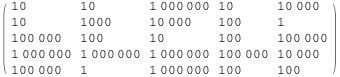
In the article Fibonacci Determinants, by Nathan Cahill et al (The College Mathematics Journal vol33 p221-225), the authors demonstrate the fact that you can obtain the nth term in the Fibonacci sequence by taking the determinant of a n x n tridiagonal matrix of the form

What’s more, if you change just a single entry (row 2 col 2) from 1 to 2 then you will obtain the Lucas Numbers instead. I thought that this was fun and so knocked up a Wolfram Demonstration for it which you can get to by clicking on the image below.

So Mr Billington – I have found yet another branch of Mathematics where the Fibonacci numbers turn up – Linear Algebra. I know it’s been 20 years but is there any chance of upping that B- to an A :) ?

If you enjoyed this article, feel free to click here to subscribe to my RSS Feed.

Here’s one for catsynth – Inspired by xkcd, Andrew J. Bennieston took a tiger into Fourier Space and back using Mathematica. The result looks kinda cool.

Wolfram Research released version 6.0.3 of Mathematica a little while ago now but, as usual, it took me a while to find the time to download and install it. Over the last month or so I have been bothering various people at Wolfram Research for more details on this new release and I am happy to say that they have been very helpful – so a big thanks to them for much of what follows. So let’s see what new goodies 6.0.3 has got compared to version 6.0.2

Possibly the most important thing you need to know about this release (if you are a Windows user) is that you should completely uninstall previous versions of Mathematica 6.x before installing 6.0.3. Exactly what might go wrong is still a mystery to me but, if I get really bored, I might try installing 6.0 side by side with 6.0.3 on a virtual machine to see what happens. If you would prefer it that everything just worked though, I suggest you take their advice.

Now that we have that out of the way – let’s look at the actual updates. One of the most visual changes is the work that Wolfram have done on the Documentation Center. There is now a comprehensive list of the standard extra packages included in the help system – something that was missing before. This gives a very useful overview of the many packages that are included with Mathematica but not loaded by default such as Combinatorica, Equation Trekker and the Vector Analysis Package. An online version of this list can be found here.

Mathematica 6.0.3 also includes quite a large number of bug fixes. In no particular order – the following have been fixed

• Under Microsoft Windows Vista there was a bug in 6.0.2 and earlier that manifested itself when you tried to print multiple copies of a notebook. The number of copies printed was the square of the number of copies selected. Version 6.0.3 prints the correct number of copies.

• On Linux, If you were running 6.0.2 or below on a compositing window manager such as Compiz then the Mathematica front end would display some inactive, blank windows. There was also a problem with the font rendering on distributions such as Ubuntu Hardy Heron and Fedora Core 9 (as described here) . This has now been fixed.

• In previous versions there was a problem with MatrixForm and TableForm in that the TableAlignment option would be ignored and everything would be aligned to the left no matter what you selected. For example in 6.0.2

  MatrixForm[10^RandomInteger[{0, 6}, {5, 5}], TableAlignments -> Center]

  

  but in 6.0.3 we get

  

  as you would expect.

• In previous versions of Mathematica 6 there was a small problem with ListPlot that can be demonstrated by the following command.

  ListPlot[{{1, 2, 3, 4}, {5}}, PlotMarkers -> {“X”, “O”}]

  

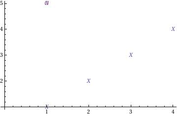
  As you can see, the O plot marker has an X plot marker superimposed over it. This has now been fixed in 6.0.3 and the above command gives the following.

  

• In 6.0.2 and earlier versions, the front end could crash in specific Manipulate outputs containing a Graphics[] expression that was selected. This is fixed in 6.0.3

• In older versions of Mathematica if you tried to import a Protein Data Bank (PDB) File that had columns with no spacing between them such as

  “ATOM 2980 C2 C B 62 10.650 -13.795-100.493 1.00 52.72 C “

  Then the import would fail. 6.0.3 fixes this.

• Pre 6.0.3, ListPlot would ignore the SetOptions command. For example – the following two commands should produce a joined up plot.

  SetOptions[ListPlot, Joined -> True];

  ListPlot[Range[50]^2]

  

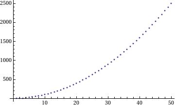
  Version 6.0.3 behaves as you would expect

  

• A minor printing bug has been fixed – In 6.0.2 and earlier 6.0 versions, no cell brackets will print even if the Print cell brackets Box is Checked in the Printing Options Dialog.

• In 6.0.2 and below the AxesLabel would overlap with the tick marks on 3D plots:

  Graphics3D[{}, BoxRatios -> {1, 1, 0.4}, Axes -> True, PlotRange -> {{0, 10}, {0, 0.4}, {0, 400}},PlotRangePadding -> Scaled[0.02], AxesLabel -> {t, x}]

  

  In 6.0.3 this has been fixed

  

• Finally, String handling in CSV file imports has changed back to the way it is documented in Mathematica. In version 6.0.2 (but not in earlier versions), if you had a CSV file that contained something like

  “hope”
  1
  2

  and you imported it into Mathematica then you would get the following result

  {{“hope”}, {1}, {2}}

  Now you get

  {{hope}, {1}, {2}}

As far as I know – that’s pretty much it. So, in a nutshell 6.0.3 is a set of bugfixes (none of them Mathematical) along with some nice documentation additions. Nothing spectacular but pretty much what one expects for such a minor release increment. Thanks to the staff at Wolfram Research who helped me out with the details on this one.

If you found this article useful, feel free to click here to subscribe to my RSS Feed

I have just returned from the 9th International Mathematica Symposium which was held in Maastricht last week where, among other things, we celebrated the 20th anniversary of the release of Mathematica. The birthday itself was on June 23rd and, as luck would have it, this was also the day of the conference dinner at the wonderful man-made caves of Geulhem so all of the IMS delegates celebrated in style. I will write more about the conference itself in a future post – once I get hold of the some of the photos.

For now, I simply wanted to highlight the fact that Wolfram have made a scrapbook that shows some of their developments over the last 20 years. We were shown a preview of it at IMS and I think there is some great material there including the complete manual for Mathematica’s predecessor, SMP (Symbolic Manipulation Program) – great for getting a flavour of how computer algebra was done in the 1980’s. While on the subject of SMP – there is a couple of screenshots of it running on a minicomputer. If you have never heard this term before you might be forgiven for thinking that a minicomputers were small, but in fact they were only small compared to the gigantic mainframes of the day. Essentially a minicomputer was the size of a two or three family washing machines as compared to the size of a house for a mainframe (or something like that – I was only 10 at the time so can’t remember!). If anyone is looking for a project, it would be very cool to get a copy of the original SMP code to work on a modern mini-computer such as a mobile phone. I wonder what the license issues are….

There are also details of the early development of the Mathematica language. What I find interesting here is how much of the early ideas survive in the present system. For me, reading code from that 20 year old dialect of Mathematica felt a little like reading victorian english – slightly odd but perfectly understandable.

I also enjoyed reading the media reactions to those early versions…one entitled “Twilight of the pencil?” by William Press for example. I find it interesting that, despite the remarkable evolution of packages such as Mathematica over the last two decades, I have yet to find a Mathematician who never does any pencil and paper maths.

I remember when I first discovered Mathematica ,version 3.0 I think it was, running on some sort of ancient Unix based system which my University had christened Newton. It was in the first month of my PhD and I had been wrestling with some terrifying looking (to a freshly minted grad student at least) integrals that were taking me ages to evaluate by hand. My PhD supervisor was a symbolic integration master and during this phase of my work I was learning loads of shortcuts and tricks that you never get taught as an undergraduate. Even with these tricks though, the work was starting to get out of hand.

One integral took me 8 A4 pages of paper to evaluate and when I took the result to my professor she glanced at it and said “that’s wrong.” For an moment I thought she already knew the answer and had just set me the problem as an exercise but she then went on to show how my result was not dimensionally consistent. A day’s work later and I had the correct answer. Over coffee someone said “There’s a package called Mathematica that could probably do those integrals – it’s installed on a machine here somewhere – maybe go and try it out.”

It took a day to find the name of the machine with Mathematica installed, another day to find said machine, 5 minutes to learn how to feed my problem to Mathematica and then about 30 seconds to reproduce several days worth of manual labour. I was in love! You would think that the pace of my research would have accelerated but I got very sidetracked learning what else I could do with my new toy.

If you have any stories concerning your early Mathematica experiences, feel free to share them in the comments section.

Oh, and the scrapbook is here – www.wolfram.com/company/scrapbook/