Walking Randomly

Here is a combination I never thought I would see – using Mathematica to update your twitter account courtesy of code from James Rohal. I’ve not tried it yet but it looks like fun!

If you have never heard of Twitter I suggest you take a look at the Wikipedia article.  It’s a lot of fun and you’ll find people like  Stephen Fry and Barack Obama among its users.

Update (12th May2009): A little while after James posted his tutorial, Wolfram Research updated their blog with a more in-depth look at accessing Twitter from Mathematica.

One of my informants told me to expect something big from Wolfram Research in the near future but didn’t tell me what it was. No matter how hard I tried, she wouldn’t give me any details apart from ‘Stephen is very excited about it‘ and ‘A surprise announcement will be coming soon.‘  She sure knows how to get me intrigued.

Well, now the secret is out…sort of.  Stephen Wolfram has just made a blog post about a project he has been working on for a few years called Wolfram Alpha.

I’ll be honest with you – I’ve read the blog post and I’m still not sure what this is all about but with phrases like:

…Fifty years ago, when computers were young, people assumed that they’d quickly be able to handle all these kinds of things. And that one would be able to ask a computer any factual question, and have it compute the answer.

and

It’s going to be a website: www.wolframalpha.com. With one simple input field that gives access to a huge system, with trillions of pieces of curated data and millions of lines of algorithms.

I am even more intrigued. Nothing is live yet – this is just an appetizer announcement but I am really looking forward to finding out more about what this is all about.

Any thoughts?

Update (18th March 2009): Doug Lenat has also seen a demo of the system and has discussed it in depth at Semantic Universe including the sort of questions that Wolfram Alpha won’t be able to answer.

John Hawks wonders if Wolfram Alpha will make bioinformatics obsolete?  I don’t know enough about bioinformatics to comment but it’s an interesting article.

Update (9th March 2009): Someone with better connections than me has seen it in action.  Check out this report for more details.

Look what I’ve got :)

News on what’s new in Mathematica 7.0.1 is sparse at the moment but I’m working on it.  The following is lifted from Wolfram’s site:

• Performance enhancements to core image-processing functions
• Right-click menu for quick image manipulation
• New tutorials, “How to” guides, and screencasts
• Thousands of new examples in the documentation
• Improved documentation search
• Integration with mathematical handwriting-recognition features of Windows 7
• Integration with the upcoming release of gridMathematica Server

Expect a follow up post soon.

When you start up Mathematica and get past the splash screen you are met with a blank screen and to a beginner* there are few things more terrifying than a blank screen.  Imagine the scene…

“What can I do?” the beginner asks

“Anything you like,” replies the master “This package gives you the ability to explore all of mathematics.  Calculus, Fourier transforms, special functions, number theory, image processing, linear algebra…all of these things and more are within your grasp.  The world is your mollusc.”

“Um..Can it plot a graph?  How do you plot the graph of sin(x) for example?” asks the beginner hopefully.

The master is somewhat deflated by this question.  He has spent much of his life learning everything there is to know about Mathematica and wants to show off his knowledge.  Hundreds of functions to choose from, hailing from every conceivable branch of Mathematics and the best this guy could do was the Sine function.  Oh well…

“Sure – that’s easy” replies the Master “Let’s start out with a simple one.  All you have to do is type the following”


Plot[Sin[x], {x, -Pi, Pi}, Ticks -> {{-Pi, -Pi/2, Pi/2, Pi}, {-1, 1}},
PlotStyle -> Red]

The beginner recoils in horror “But..but that’s PROGRAMMING. I’m not a programmer – I can’t do that kind of stuff. All I want to do is plot a graph.  Can’t I just use Excel…?”

I have used Mathematica for a few years now (ever since 2000 if you’re counting) and so I can either remember or work out the syntax for commands like the one above with relative ease but I have taught enough beginners courses to know that the above scenario isn’t too far from the truth for many people.  Learning Mathematica syntax can be a very daunting prospect if you have never done any programming before in your life.

Many students these days are much more used to clicking on buttons in a user interface to get a job done rather than typing in strings of commands.  This is where the new classroom assistant comes in very useful.

The basic idea behind the classroom assistant is that you can look through the palette for what you want to do and when you click on the relevant button it will create a template for the command in a Mathematica notebook. For example, click on Plot and you get

All the user has to do now is fill in the blanks.  What could be easier?  For more detailed information concerning the Mathematica classroom assistant check out the recent Wolfram Research blog article written by Eric Schulz – the creator of this great new tool.  If you would prefer a user’s perspective then take a look at the article written a while back by Maria of TCMTB.

*terrifying to more experienced people too for that matter

Someone at my university reported the following Mathematica 7 bug to me and I thought I would share it with all of you in case someone was interested or could offer insight that we don’t have.  Needless to say this has been reported to Wolfram via the official channels and I am sure that it will be sorted out soon.

If you do

Integrate[k^2 (k^2 – 1)/((k^2 – 1)^2 + x^2)^(3/2), {k, 0, Infinity},Assumptions -> x > 0]

you get

EllipticK[(2*x)/(-I + x)]/(2*Sqrt[-1 – I*x])

Which is complex for all x whereas the integrand is purely real.  As a  particular example let us put x=2.  Evaluating numerically:

NIntegrate[k^2 (k^2 – 1)/((k^2 – 1)^2 + 2^2)^(3/2), {k, 0, Infinity}]

gives

0.706094

But if I plug x=2 into the symbolic result given earlier

N[EllipticK[(2*x)/(-I + x)]/(2*Sqrt[-1 – I*x]) /.x->2]

Then I get

-5.35054*10^-17 + 0.568541 I

Which is obvioulsy incorrect.  Would someone with a copy of Maple 12 mind seeing what that makes of this integral please?  Extra kudos to anyone who can do it by hand!

The Wolfram Demonstrations project has been updated to take advantage of the new features of version 7 of Mathematica and Jeff Bryant has written a great post about it on the Wolfram Research Blog.  As you might expect, Wolfram have also upgraded their free Mathematica player which allows you to run all of their demonstrations without a Mathematica license.

Some of the new demonstrations are very pretty!  I particularly like their new vector field plotting routines as shown in the demonstration below which calculates the electric field pattern formed by three point charges.

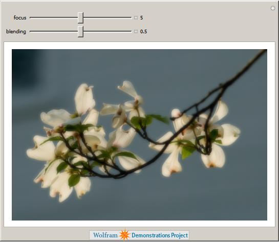
The new image processing routines that Wolfram have added to Mathematica allow for the easy production of some very beautiful demonstrations.  Here is one by Peter Overmann that simulates a photographic technique called the Orton Effect.

Mathematica 7 includes some very nice support for parallel computing and one of the easiest commands to use is Parallelize.  If you have a multi-core computer (and most of them are these days) then, in some cases, you can get a speedup of a factor of 2 or more simply by wrapping your code with the Parallelize command.  I’ll stress that it’s not always this easy but, when it is, it’s very nice.

To start getting my head around the new command I looked at the following small piece of code which is included in the Mathematica 7 documentation.

data = Table[ PrimeQ[n! + 1], {n, 400, 550}];

This code calculates numbers of the form n!+1 for n between 400 and 550 and tests to see if they are prime or not. Let’s see how long it takes on my dual core 2Ghz Dell XPS M1330:

data = Table[ PrimeQ[n! + 1], {n, 400, 550}]; // AbsoluteTiming

Out[1]={14.092809, Null}

We see from the above that it took just over 14 seconds before we apply any parallelism. Let’s see how much improvement we get by using the Parallelize command:

data = Parallelize[Table[ PrimeQ[n! + 1], {n, 400, 550}]]; // AbsoluteTiming
Out[2]= {21.124572, Null}

Oh dear, something has gone drastically wrong! The parallel calculation is taking 7 seconds (or 50%) longer than the serial calculation. Before writing a bug report to Wolfram, I thought I would dig around a little to try and work out what was going on.

First things first, let’s take a look at how hard Mathematica is pushing the processor in both cases.  I can add a little CPU monitoring applet to my GNOME panel by right clicking on it and selecting add to Panel.  From the resulting list I choose CPU Frequency Scaling Monitor.

When I initially did this, the applet informed me that my CPU was running at 800 Mhz – way below its maximum speed of 2Ghz.  When I click on this applet I get a range of settings that could be applied to my CPU such as On demand, Performance and Powersave along with specific speed settings from 800Mhz to 2 Ghz. The one selected was on demand.

Turning back to Mathematica I run the sequential code again

data = Table[ PrimeQ[n! + 1], {n, 400, 550}]; // AbsoluteTiming
Out[3]={14.117028, Null}


According to the CPU Monitor, my computer was running at 2Ghz (its top speed) during the entire calculation. However, when I ran the Parallelize version, the processor speed remained at 800Mhz the whole time. So, the calculation may well have been running in parallel but each of the 2 cores was only running at 40% of top speed.  The problem seems to lie with Mathematica’s interaction with the on demand setting of the processor manager.

By clicking on the GNOME CPU monitor, I can fix the processor to run at 2Ghz at all times – no fancy processor management here – just the fastest speed my computer can manage.  Let’s see what the results of the two versions of the code are when I do this.

data = Table[ PrimeQ[n! + 1], {n, 400, 550}]; // AbsoluteTiming

Out[4]={14.062377, Null}

data = Parallelize[Table[ PrimeQ[n! + 1], {n, 400, 550}]]; // AbsoluteTiming

Out[5]={7.635570, Null}

That’s more like it! The parallel version is almost twice as fast as the serial version – just as we would expect on a dual core system. So, the moral of the story is to ensure that you don’t have your system set to modify it’s processor speed on demand when trying to make use of the new Parallel features of Mathematica 7.

For the record I am running GNOME 2.24.1 on Ubuntu 8.10 with Mathematica 7.

Version 7 of Wolfram Research’s flagship product, Mathematica, has been released today – just 18 months after version 6.  I have been fiddling with beta versions of it for a while now and have been desperate to start talking about it but the NDA I signed prevented me from doing so until today.

A full review will have to wait because, paradoxically, I don’t have access to the full version of Mathematica 7 right now but here are a few highlights that got my attention during beta testing.

Built in Parallel Computing

The computer I am typing this blog post on is nothing special by today’s standards and yet it is a quad-core machine which effectively means that it contains not 1 but 4 CPUs.  Most pieces of software tend to only use one of these cores which means that the other 3 are sitting about doing nothing most of the time.  It’s a bit like being assigned a team of helpers to help you work on a project and then saying to 3 of them – “You guys can just sit around doing nothing  because I don’t know how to use you.”  Pretty shoddy management huh?  Ideally, what you need to do is to parallelize your algorithm so those other 3 cores can get off their backsides and do something useful.

Previous versions of Mathematica had limited support for making use of multi-core machines like mine.  As far as I know they were limited to relatively low level matrix and vector operations that made use of underlying BLAS and LAPACK libraries.  I had a brief forum discussion with some people on this topic a while back but never got around to following it up.

If you wanted to write fully parallel code with previous versions of Mathematica then you needed to buy a separate product called the Parallel Computing Toolkit.  Most people who expressed an interest in parallel Mathematica at my university soon lost interest when they realised that they would have to spend more money to make it work.

In Version 7, Wolram have done the right thing and have built in a whole suite of commands and frameworks to allow you to fully parallelize your Mathematica code.  Now, finally, you can make use of the spare cores in your computer.  There will be follow up blog posts on this topic I can assure you (just as soon as I figure out how to do it all!)

Image Processing

While at the International Mathematica Symposium in Maastricht I saw my first demonstration of version 7 and one of the things that caught my attention was the range of image processing features that Wolfram were building into the product.  In the demonstration, the speaker was manipulating photographs in Mathematica exactly as you might manipulate any other mathematical expression.  In other words you could give the photograph itself as the argument to a function!  There was no messing around with file handles or input streams or whatever – you just wrapped the picture in a function and pressed enter.  For example (images used with permission from Wolfram Research) – The following input

Gives the following output

Wolfram have also added a whole suite of image manipulation algorithms and so with just a few commands even someone like me (who knows nothing about image processing) could write fully interactive image processing applications.  I imagine that this would be extremely useful for the academics I work for as well as being a lot of fun for me (can anyone recommend a good book that teaches about image processing algorithms by the way).

Delay Differential Equations

Mathematica now has built in support for delay differential equations and my boss used to do research into these a few years ago so we’ll have yet another topic to talk about.  I note that MATLAB has support for these too and so a future comparison might be interesting.

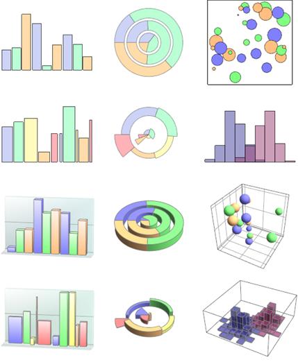
Improved charting

Mathematica has always been able to do things like Pie charts, bar charts and the like but they have never been as good as other areas of Mathematica’s plotting functionality such as 2 and 3D function plots.  In version 7, this area of visualization has been vastly improved.

More, More more

Version 7 is the first major version of Mathematica that I have covered since starting this blog and I have to say I am a little overwhelmed with the quantity of improvements that Wolfram have made.  Up until now I have only talked about minor releases such as 6.0.3 and 6.0.2 where I could cover pretty much all of the new functionality in a single blog post – with version 7 I have no chance.  There is just too much to include all at once.

Finally, my friend Maria over at TCMTB has discussed a new Mathematica 7 feature that I wasn’t even aware of: The Classroom Assistant.  Head over there to see what she has to say about it.

Expect to see a lot more in-depth articles about Mathematica 7 on Walking Randomly in the future.  Any requests?

The Wolfam Demonstrations project has just topped 4000 submissions! I make no secret of the fact that I love the Wolfram Demonstrations project and barely a day goes by where I don’t mention it to someone. It’s got so bad that I am sometimes accused of being a secret employee of Wolfram Research (I’m not – just for the record – but they are free to make me an offer.) If you are new around here then here is a quick summary of why I like it so much.

• Over 4000 demonstrations covering a very wide range of disciplines.
• Every demonstration is fully interactive and can be used for free via the Mathematica player.
• Full Mathematica source code for every demonstration is easily available. So, if you have a full copy of Mathematica then you can modify them for your own purposes.
• Everyone who has a fully licensed copy of Mathematica can contribute. This is a true community project.
• The guys and gals at Wolfram vet each and every one of the submissions to ensure that they meet various guidelines. If you are an author of a demonstration then they give advice on how you might improve your submission. Sometimes they even supply code that you might not have been able to come up with yourself.

In my opinion, the project really is all things to all people. For example, if you are a teacher then you might use some of the demonstrations to spice up your courses at no cost. Remember – you can download the free Mathematica Player and use all of the demonstrations fully interactively. There is no need to buy a Mathematica license! I often hear maths educators say “The only way to learn mathematics is to do mathematics.” and they are absolutely right! The Wolfram Demonstrations project gives you and your students another way to ‘do math’. Have you just taught some Fourier analysis? Well then, you might be interested in some examples of Fourier Series or maybe you would like to discuss (and demonstrate) Fourier sound synthesis. You might decide to demonstrate how the Fourier Transform can be used for image compression or maybe show the problems that Fourier series have with discontinuites.

If none of the demonstrations do quite what you want then download the source code and modify them. If you don’t have a full copy of Mathematica or the required programming skills then send a request to Wolfram and they may be able to help. Alternatively ask me – I’ll help whenever I can and have done so in the past both for readers of this blog and for teachers and researchers at my place of work (The University of Manchester).

If you are learning how to use Mathematica and prefer to learn from examples then the project is perfect. 4000+ real-world examples right at your fingertips. For free! I have used Mathematica for over 8 years now and yet I constantly come across new techniques and ideas by reading the source code of other author’s submissions.

Perhaps you are not a programmer or a teacher and you just like fiddling around with Mathematics? Again, the Wolfram Demonstrations project is for you. You might choose to play a relaxing game of Tangrams or challenge your brain with Sudoku. Alternatively you be interested in some of the mathematics behind prime numbers or perhaps you want to play around with polygonal numbers?

So, what would you like to see? Although there are over 4000 different demonstrations so far, there is still a lot of stuff left to cover. What is your personal wish list for the Demonstrations project? If you ask you might get ;)

If you enjoyed this article, feel free to click here to subscribe to my RSS Feed.

One comment about my recent review of the new symbolic toolbox for MATLAB 2008b was that I didn’t mention any bugs. To be fair to me I simply didn’t know of any back then but things change so here is one for your viewing pleasure. The following problem with the solve command was originally mentioned on the matlab newsgroup a few days ago.

solve ('x^(5/2) + x^(1/2) = 42')

ans =
0

The solution should have been as follows (found with version 2007b of MATLAB and the symbolic toolbox)

ans =
4.3694949188853387526809476648368
-3.5354997083462823180109844585991-2.6744595794528774961538687374412*i
-3.5354997083462823180109844585991+2.6744595794528774961538687374412*i


Mathworks are aware of the problem and I am sure a fix will be released soon. So why have I chosen to focus on this you may ask?

Well, I have a rather strange relationship with bugs like this in computer algebra software in that I think that they are immeasurably useful! I love finding bugs in programs like MATLAB and Mathematica and will often make as much noise as possible about them. Is this because I hate the likes of Wolfram Research and Mathworks? Do I want to rip into them at every possible opportunity? Do I enjoy seeing big companies fail?

Not even close. Quite the opposite in fact.

Systems such as Mathematica and MATLAB seem almost impossibly powerful – they can do calculations that are far beyond my feeble little mind and they can do plenty of things beyond the ken of much more powerful minds too. It’s very tempting to take whatever results they spit out and present them as the correct answer. Always. All the time. Without exception. Mathematica/MATLAB gives this or that answer so it must be true! Right?

Wrong! So wrong that I go a funny shade of red whenever I see this opinion being expressed. Computer programs are developed by ordinary, everyday people just like you and me. They just happen to be rather good at programming computers. People make mistakes so we should expect that the programs they create will make mistakes too. This is no big deal and is nothing to lose sleep over – it’s just the way things are. I make mistakes, you make mistakes and Shock! Horror! MATLAB makes mistakes too.

Once you know and accept this you simply factor it into the way you work. When you plug a problem into Mathematica or MATLAB make sure that you think about the result you expect to get. Does the output look reasonable or is it clearly a load of old hogwash? If it does look reasonable then can you compute it via another method to check that there is nothing wrong with the first algorithm you tried?

How much does the correct result matter? If it is a matter of life and death then check it again and again. Then once more just for good measure. If it doesn’t matter so much then maybe check it just the once – or maybe not at all if it’s no big deal. Just be aware that it might be wrong.

There is no need to be too concerned though since one of the reasons why bugs like the one above are so interesting is that they are actually quite rare. I can sit in front of MATLAB day after day and never uncover a single bug – it’s pretty good at what it does to be fair. So…you can safely trust MATLAB – most of the time at least :)

I think that the occasional bug or two is good for the soul as they remind us that nothing is infallible – not even programs like MATLAB and it’s almost a shame that The Mathworks fixes them so quickly. So…go forth and find bugs. Don’t be afraid of them but learn from them. When you do find one, please tell me all about it though as I love a good bug! It’s probably best to tell the vendor about it too though, after all they are the ones who can fix it.

Finally, if anyone from The Mathworks or Wolfram Research is reading this, then I have a request if I may. Take a look through your bug database and try to pick out a really juicy one for us. It could be a symbolic integral that your system couldn’t do or maybe a numerical result that is so far from being correct it’s not even funny. Why did your program fail with that particular problem? If it is a straightforward programming bug then it’s probably not very interesting to the general reader but if there is something tricky about the mathematics that you had to overcome then I bet there will be a lot of people who would be interested in hearing about it.

Me for one!

If you enjoyed this article, feel free to click here to subscribe to my RSS Feed.