Walking Randomly

A Mathematica user contacted me recently and asked why

(1/16 Cos[a] (Cos[b] + 15 Cos[3 b])) === (1/8 Cos[b] (-7 + 15 Cos[2b])Cos[a])

returned False when he expected True. Let’s take a look at what is going on here.

The SameQ command (===) and the Equal command (==) are subtly different.  Equal (==) tests to see if two expressions are mathematically equivalent whereas SameQ tests to see if they are structurally equivalent.  In general, SameQ is the stricter of the two tests and is often too strict for our needs.

A very simple example

The simplest example might be to compare 2 and 2. (That is 2 with a period at the end)

Mathematically these are the same since they both represent the number two. However, from a Mathematica structural point of view, they are different since one has infinite precision whereas the other has double precision. So, we have

2==2. gives True
2===2. gives False

A more complicated example

Sqrt[2] + Sqrt[3] == Sqrt[5 + 2 Sqrt[6]] which gives True
Sqrt[2] + Sqrt[3] === Sqrt[5 + 2 Sqrt[6]] which gives False

Mathematically the above is always true but the structure of the expressions on the LHS and RHS are different under normal evaluation rules.

So, what do I mean by ‘structurally equivalent?’.  To be honest, I am slightly woolly on this myself but in my head I consider two expressions to be structurally equivalent if their TreeForms are the same

TreeForm[Sqrt[2] + Sqrt[3] ]

TreeForm[Sqrt[5 + 2 Sqrt[6]] ]

The important thing to remember here is that the argument to TreeForm is evaluated by Mathematica before it gets passed to TreeForm. So, the above images show us that under normal evaluation rules, these two expressions have different structural forms.  In the next example we’ll see how this detail can matter

Exp[I Pi] and all that

Let’s look at

Exp[I Pi] === -1

Would that be True or False based on what we have seen so far?  It is certainly mathematically true but remember that a triple equals requires both sides to be structurally equivalent and at first sight it appears that this isn’t the case here. You might expect Exp[I Pi] to have a very different TreeForm from -1 and so you’d expect the above to evaluate to False. However if you do

TreeForm[Exp[I Pi]]

then you get a single box containing -1. This occurs because Mathematica evaluates Exp[I Pi] to -1 before passing to TreeForm. This evaluation also occurs when you do Exp[I Pi] === -1 so what you are really testing is -1===-1 which is obviously True.

Back to the original example

(1/16 Cos[a] (Cos[b] + 15 Cos[3 b])) === (1/8 Cos[b] (-7 + 15 Cos[2b])Cos[a])

If you use === then it returns False and this is ‘obviously’ the case because if you evaluate the TreeForms of both expressions then you’ll see that they get stored with different structural forms after being evaluated.

TreeForm[(1/16 Cos[a] (Cos[b] + 15 Cos[3 b]))]

TreeForm[(1/8 Cos[b] (-7 + 15 Cos[2 b]) Cos[a])]

Since we are interested in mathematical equivalence, however, we use ==

(1/16 Cos[a] (Cos[b] + 15 Cos[3 b])) == (1/8 Cos[b] (-7 + 15 Cos[2 b]) Cos[a])

What happens this time, however, is that Mathematica returns the original expression unevaluated. This is because, under the standard set of transformations that Mathematica applies when it evaluates ==, it can’t be sure one way or the other and so it gives up.

To proceed we wrap the whole thing in FullSimplify which essentially says to Mathematica ‘Use everything you’ve got to try and figure this out – no matter how long it takes’  I.e. you allow it to use more transforms.

FullSimplify[(1/16 Cos[a] (Cos[b] + 15 Cos[3 b])) == (1/8 Cos[b] (-7 + 15 Cos[2 b]) Cos[a])]

True

Finally, we have the result that the user expected.

MATLAB’s control system toolbox has functions for converting transfer functions to either state space representations or zero-pole-gain models as follows

%Create a simple transfer function in MATLAB
num=[2 3];
den = [1 4 0 5];
mytf=tf(num,den);

%convert this to State Space form
tf2ss(num,den)
ans =

0   1   0
0   0   1
-5  -0  -4

%Convert to zero-pole-gain form
[z,p,k]=tf2zp(num,den)
z = -1.5000
p =

-4.27375 + 0.00000i
0.13687 + 1.07294i
0.13687 - 1.07294i

k =  2

Now that Mathematica 8 is available I wondered what the Mathematica equivalent to the above would look like. The conversion to a StateSpace model is easy:

mytf=TransferFunctionModel[(2 s + 3)/(s^3 + 4 s^2 + 5), s]
StateSpaceModel[mytf]

but I couldn’t find an equivalent to MATLAB’s tf2zp function.

I can get the poles and zeros easily enough (as an aside it’s nice that Mathematica can do this exactly)

TransferFunctionPoles[mytf]
TransferFunctionZeros[mytf]

but what about gain?  There is no TransferFunctionGain[] function as you might expect. There is a TransferFunctionFactor[] function but that doesn’t do what I want either.

It turns out that there is a function that will do what I want but it is hidden from the user a little in an internal function

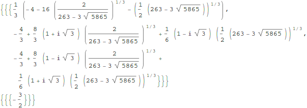
Control`ZeroPoleGainModel[mytf]

Control`ZeroPoleGainModel[{{{{-(3/2)}}}, {1/
     3 (-4 - 16 (2/(263 - 3 Sqrt[5865]))^(
        1/3) - (1/2 (263 - 3 Sqrt[5865]))^(1/3)), -(4/3) +
     8/3 (1 + I Sqrt[3]) (2/(263 - 3 Sqrt[5865]))^(1/3) +
     1/6 (1 - I Sqrt[3]) (1/2 (263 - 3 Sqrt[5865]))^(1/3), -(4/3) +
     8/3 (1 - I Sqrt[3]) (2/(263 - 3 Sqrt[5865]))^(1/3) +
     1/6 (1 + I Sqrt[3]) (1/2 (263 - 3 Sqrt[5865]))^(1/3)}, {{2}}}, s]

That’s not as user friendly as it could be though. How about this?

tf2zpk[x_] := Module[{z, p, k,zpkmodel},
  zpkmodel = Control`ZeroPoleGainModel[x];
  z = zpkmodel[[1, 1, 1, 1]];
  p = zpkmodel[[1, 2]];
  k = zpkmodel[[1, 3, 1]];
  {z, p, k}
  ]

Now we can get very similar behavior to MATLAB:

In[10]:= tf2zpk[mytf] // N

Out[10]= {{-1.5}, {-4.27375, 0.136874 + 1.07294 I,
  0.136874 - 1.07294 I}, {2.}}

Hope this helps someone out there.  Thanks to my contact at Wolfram who told me about the Control`ZeroPoleGainModel function.

Other posts you may be interested in

• Mathematica 8 – Control Theory Sneak Peek
• 5 new plot commands in Mathematica 8

I thought I’d try out the new image capturing functionality in Mathematica 8 on my Linux based laptop with built in webcam but…

In[1]:= ImageCapture[]
During evaluation of In[1]:= ImageCapture::notsupported: Image acquisition is not supported on Unix. >>
Out[1]= ImageCapture[]

That makes me a sad panda!

Version 8 of Mathematica was released on Monday 15th November and it’s a big one!  With permission from Wolfram Research , I’ve been releasing little preview snippets from the beta version over the last couple of months but they hardly scratch the surface.  I’m really excited about this release and so rather than post a traditional review of the product in a couple of weeks time, I thought that I’d try something different.

The idea is that this post will grow with new information and observations on the new version as they happen.  One of the things I’ll be focusing on is the new Wolfram portal for site license administrators in the hope that it might help other unlimited site administrators.

So, if you have anything to say about version 8 then post your comments, links and code here.

10th March 2011 – Wolfram Portal Problems Fixed

I am very pleased to be able to report that almost all of the issues I had with Wolfram’s portal have been fixed and Manchester University is beginning the Mathematica 8.0.1 roll-out to its staff and students.  A huge thank you to the Wolfram portal staff who have been working with me on this.

9th March 2011 – Wolfram Demonstrations Site Overhauled.  CDF Player launched.

Check out Wolfram’s blog post on this at http://blog.wolfram.com/2011/03/08/innovating-interactive-web-publishing-with-wolfram-demonstrations/.  See one of the first interactive .cdf (computable document format) demonstrations outside of Wolfram Research at Mathematica: Interactive mathematics in the web browser

7th March 2011 – Mathematica 8.0.1 has been released

In an email to me Wolfram say ‘Mathematica 8.0.1 includes more than 500 improvements, including feature, stability, and performance enhancements, as well as documentation updates.’ Sadly there is no indication of what any of these changes actually are!  That sucks!

10th December 2010 – Wolfram Portal Problems

When I first saw the new Wolfram Portal, I thought that it would make my life as a license administrator (and the lives of my colleagues) much easier and that I would be able to release Mathematica 8 to our University in double quick time.  Sadly, however, it has not lived up to expectations and I now feel that it has some serious problems that need fixing before we start using it in anger.  I don’t want to go into details just yet because I’m working with Wolfram to try to come to a resolution.

For now, however, I am sad to report that Manchester University won’t be rolling out Mathematica 8 to the masses for a while yet.

20th November

• Just discovered that Image capture is not supported on Linux machines.
• Some people have asked me if Mathematica 8 has improved ‘undo’ functionality.  The answer is no – undo is identical to v7 (as far as I can tell).

18th November

Some new Mathematica 8 coverage:

• How many MATLAB toolboxes make a Mathematica 8? I wrote this out of curiosity.  The list is longer than I expected.
• Programming with Natural Language is Actually Going to Work. Stephen Wolfram discusses the new NLP features in Mathematica.  I have to say that it’s a feature I find myself using more and more.  I don’t like leaving natural language in my notebooks though – it just looks wrong to my eyes and I worry that the behaviour of my notebook may change if Wolfram were to modify the Wolfram Alpha back-end.  It is, however, a great way of quickly looking up Mathematica syntax and that’s mostly how I use it right now.

17th November 11:00
Some issues with Wolfram’s new site license administration portal are as follows

• Downloads are much slower than people would like.  My beta testers have already requested that we host the Mathematica 8 installers on our local university servers.  I’ve officially requested this from Wolfram. (fixed)
• It is not possible to use email wildcards when specifying who can request licenses or not.  For example, if the requesters email doesn’t end with @manchester.ac.uk (and variants) then I want it to be automatically rejected with a message of our choice.  Sadly I cannot do this which means that we’ll be doing lots of rejections from people who we can’t easily verify are are members of our university. (fixed)
• The site license admins get an email every single time someone requests a license from us.  A once a day digest would be much more useful!

16th November 15:50
I have my own copy of Mathematica 8 up and running and I’ve started playing with it a little.  Just tried the following two commands on my desktop machine to see if I can get the CUDA interface working

Needs["CUDALink`"]
CUDAInformation[]

Mathematica 8 needs to load something from Wolfram’s servers in order to complete this command and it’s taking an age. Several minutes in and it’s only at 17%. I guess Wolfram’s servers are being hammered right now (either that or there’s a local network problem). Definitely a down-side of cloud-based computing.

16th November 15:00

A colleague and I have been poking around the new Wolfram site license administrators portal and overall we are impressed.  There are a few issues to iron out before we feel confident enough to open Mathematica 8 to all Mathematica users at Manchester but the system appears to be a vast improvement on what has gone before.  This may be the fastest release to site I have ever performed.  Sent Wolfram tech support about a trillion questions (sorry guys!)

16th November 12:30

Our site license has been upgraded already!  Now to get my head around the new portal and see what needs to be done to get the goodies out to Manchester Uni users.

16th November 10:30

My employer, The University of Manchester, has a full site license for Mathematica and I am one of the administrators of this license.  I’ve already had my first request from a user who wants to upgrade to version 8 (very keen these Mathematica users) but Wolfram haven’t yet upgraded the site license from version 7.0.1.  So, even I, as the administrator of an unlimited site license can’t get my hands on the goodies yet.  Hopefully this will change soon because we’ve got a lot of work to do internally before we release it to our site.

16th November 09:00

I’ve just read Stephen Wolfram’s blog post about the new free-form linguistics in Mathematica 8.  It all looks very awesome but it seems that Wolfram Alpha is used to process the free-form input.  This leads me to wonder about the following questions

• How much of the free-form linguistic functionality will you get if you are offline?
• Will any information about the user be sent to and kept by Wolfram Research?  If nothing else then I guess this will give Wolfram some very detailed usage information.
• Since it has to go across the Internet to do some of the processing, how much will using free-form input slow things down?

Mathematica 8 around the web

• The Owen’s T function
• Symbolics and Numerics combine to form new integration Algorithm
• Mathematica, CUDA and GPUs
• Real time image capturing
• 5 new plot commands in Mathematica 8
• Control Theory Sneak Peek

Christmas isn’t all that far away so I thought that it was high time that I wrote my Christmas list for mathematical software developers and vendors.  All I want for christmas is….

Mathematica

• A built in ternary plot function would be nice
• Ship workbench with the main product  please
• An iPad version of Mathematica Player

MATLAB

• Merge the parallel computing toolbox with core MATLAB.  Everyone uses multicore these days but only a few can feel the full benefit in MATLAB.   The rest are essentially second class MATLAB citizens muddling by with a single core (most of the time)
• Make the mex interface thread safe so I can more easily write parallel mex files

Maple

• More CUDA accelerated functions please.  I was initially excited by your CUDA package but then discovered that it only accelerated one function (Matrix Multiply).  CUDA accelerated Random Number Generators would be nice along with fast Fourier transforms and a bit more linear algebra.

MathCAD

• Release Mathcad Prime.
• Mac and Linux versions of Mathcad.  Maple,Mathematica and MATLAB have versions for all 3 platforms so why don’t you?

NAG Library

• Produce vector versions of functions like g01bk (poisson distribution function).  They might not be needed in Fortran or C code but your MATLAB toolbox desperately needs them
• A Mac version of the MATLAB toolbox.  I’ve got users practically begging for it :)
• A NAG version of the MATLAB gamfit command

Octave

• A just in time compiler.  Yeah, I know, I don’t ask for much huh ;)
• A faster pdist function (statistics toolbox from Octave Forge).  I discovered that the current one is rather slow recently

SAGE Math

• A Locator control for the interact function.  I still have a bounty outstanding for the person who implements this.
• A fully featured, native windows version.  I know about the VM solution and it isn’t suitable for what I want to do (which is to deploy it on around 5000 University windows machines to introduce students to one of the best open source maths packages)

SMath Studio

• An Android version please.  Don’t make it free – you deserve some money for this awesome Mathcad alternative.

SpaceTime Mathematics

• The fact that you give the Windows version away for free is awesome but registration is a pain when you are dealing with mass deployment.  I’d love to deploy this to my University’s Windows desktop image but the per-machine registration requirement makes it difficult.  Most large developers who require registration usually come up with an alternative mechanism for enterprise-wide deployment.  You ask schools with more than 5 machines to link back to you.  I want tot put it on a few thousand machines and I would happily link back to you from several locations if you’ll help me with some sort of volume license.  I’ll also give internal (and external if anyone is interested) seminars at Manchester on why I think Spacetime is useful for teaching mathematics.  Finally, I’d encourage other UK University applications specialists to evaluate the software too.
• An Android version please.

How about you?  What would you ask for Christmas from your favourite mathematical software developers?

If you love your code…set it free!  That’s what Will Robertson did when he released the first version of colorbarplot for Mathematica.  I liked what he did but it didn’t do quite enough for my needs so I added some stuff to it and a new version was born.

Our package starting getting users and some of those users asked for things so Will and I added yet more stuff and colorbarplot version 0.5 was born.

Finally, one of those users, Thomas Zell of the University of Cologne, has added more functionality of his own resulting in version 0.6 of colorbarplot.  So, what’s new?

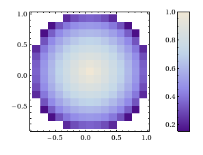
Well, if you have data in the form of a two-dimensional array, in which not every entry has valid numerical data, the following will now work without error:

set1 = Table[
   If[Sqrt[x^2 + y^2] < 1, Sqrt[1 - Sqrt[x^2 + y^2]]], {x, -1, 1,      0.125}, {y, -1, 1, 0.125}];
ColorbarPlot[set1, InterpolationOrder -> 0,
 DataRange -> {{-1, 1}, {-1, 1}}]

Next up, if you want to compare two data sets, the plots have to have the same scale even if the data sets have different sizes. This can now be achieved with the PlotRange option:

set2 = Table[
  If[Sqrt[x^2 + y^2] < 2, Sqrt[2 - Sqrt[x^2 + y^2]]], {x, -2, 2,    0.125}, {y, -2, 2, 0.125}]; 

{ColorbarPlot[set1, InterpolationOrder -> 0,
 DataRange -> {{-1, 1}, {-1, 1}},
 PlotRange -> {{-2, 2}, {-2, 2}, {0, 1.5}}],
ColorbarPlot[set2, InterpolationOrder -> 0,
 DataRange -> {{-2, 2}, {-2, 2}},
 PlotRange -> {{-2, 2}, {-2, 2}, {0, 1.5}}]}

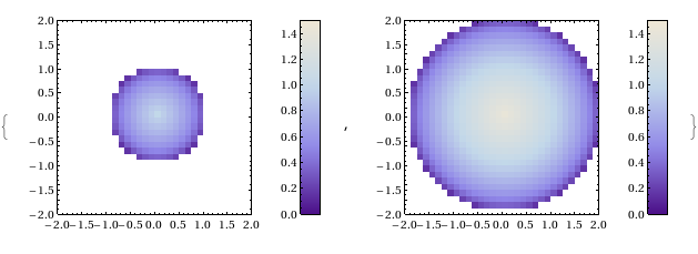
This is great stuff, helps make colorbarplot more useful and turns the package into a truly international collaboration ;)

• ColorbarPlot’s github page The latest version will always be available here
• ColorbarPlot’s page in the Wolfram Library This is often out of date.
• ColorbarPlot 0.6 from the WalkingRandomly server
• ColorbatPlot 0.5 My write up of a previous version
• ColorbarPlot 0.4 My write up of a previous version
• ColorbarPlot 0.3 My write up of a previous version

Have you published anything that uses colorbarplot?

If you have published anything that uses our little package then please do let us know.  We know we have users so it would be great to see how you are using it.  The more feedback we get, the more likely we are to want to develop it further.

Mathematica 8 is coming and it’s chock-full of new features.  Last month I took a very brief look at some of the new control systems functionality that we’ll be getting and this time around I thought I would take a look at some of the new plotting functions.

The first new command that I’d like to show you is a revamped box and whisker plot. Mathematica 7 could do these as part of the StatisticalPlots package but they seemed a bit of an afterthought and didn’t have many options.

Needs["StatisticalPlots`"]
data1 = RandomReal[NormalDistribution[0, 1], 100];
data2 = RandomReal[{0, 1}, 100];
BoxWhiskerPlot[data1, data2]

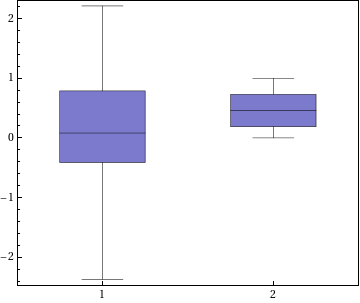
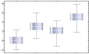
The above code still works in Mathematica 8 but you’ll be told that it’s obsolete. The new way of doing things is to use BoxWhiskerChart which looks better, has a boat load of new options and also comes with a very nice tool-tip.

data = Table[
   RandomVariate[NormalDistribution[mu, 1],
    100], {mu, {0, 3, 2, 5}}];
BoxWhiskerChart[data, ChartElementFunction -> "GlassBoxWhisker"]

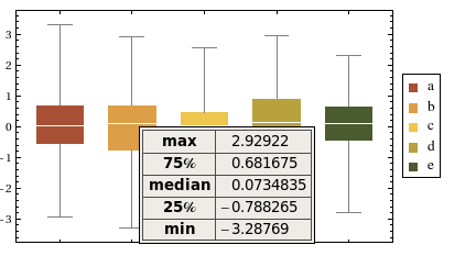
BoxWhiskerChart[RandomVariate[NormalDistribution[], {5, 100}],
 ChartStyle -> "SandyTerrain",
 ChartLegends -> {"a", "b", "c", "d", "e"}]

Next up is something from the world of Finance – a Kagi Chart.

data = FinancialData["L:LLOY",
   "Close", {{2010, 6, 1}, {2010, 11, 1}, "Day"}];
KagiChart[data, TrendStyle -> {Green, Red}]

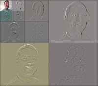
How about some wavelets? Let’s do a discrete wavelet transform of a photo of me and use WaveletImagePlot to show the wavelet image coefficients.

me = Import["me.jpg"];
dwd = DiscreteWaveletTransform[me, Automatic, 3];
WaveletImagePlot[dwd, ImageSize -> 200]

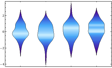
Next up is a plot-type that is completely new to me – A violin plot.

DistributionChart[RandomVariate[NormalDistribution[0, 1], {4, 100}],
 ChartElementFunction ->
  ChartElementData["SmoothDensity", "ColorScheme" -> "DeepSeaColors"]]

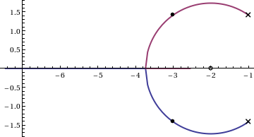
Finally, A little more control systems with a Root Locus Plot.

RootLocusPlot[
 StateSpaceModel[{{{0, 1}, {-3, -2}}, {{0}, {1}}, k {{2, 1}}}], {k, 0,
   8}]

What I like most about all of these new plot types is that they will be built in to core Mathematica as of version 8 – no add-ons necessary. Compare this to MATLAB which has functions for most of the above plots but only if you buy the relevant toolbox:

• Box and Whisker Plot – Statistics Toolbox
• Kagi Chart – Finance Toolbox
• Wavelet coefficients – Wavelet Toolbox
• Root locus plot – Control Systems Toolbox
• Violin Plot – ?????

I much prefer Mathematica’s all in one approach and I am really looking forward to this release.  Thanks to Wolfram Research for allowing me to release this little preview.

How about you?  What plot types are you hoping for in Mathematica 8?

Some time ago now, Sam Shah of Continuous Everywhere but Differentiable Nowhere fame discussed the standard method of obtaining the square root of the imaginary unit, i, and in the ensuing discussion thread someone asked the question “What is i^i – that is what is i to the power i?”

Sam immediately came back with the answer e^(-pi/2) = 0.207879…. which is one of the answers but as pointed out by one of his readers, Adam Glesser, this is just one of the infinite number of potential answers that all have the form e^{-(2k+1) pi/2} where k is an integer. Sam’s answer is the principle value of i^i (incidentally this is the value returned by google calculator if you google i^i – It is also the value returned by Mathematica and MATLAB). Life gets a lot more complicated when you move to the complex plane but it also gets a lot more interesting too.

While on the train into work one morning I was thinking about Sam’s blog post and wondered what the principal value of i^i^i (i to the power i to the power i) was equal to. Mathematica quickly provided the answer:

N[I^I^I]
0.947159+0.320764 I

So i is imaginary, i^i is real and i^i^i is imaginary again. Would i^i^i^i be real I wondered – would be fun if it was. Let’s see:

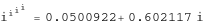
N[I^I^I^I]
0.0500922+0.602117 I

gah – a conjecture bites the dust – although if I am being honest it wasn’t a very good one.  Still, since I have started making ‘power towers’ I may as well continue and see what I can see. Why am I calling them power towers? Well, the calculation above could be written as follows:

As I add more and more powers, the left hand side of the equation will tower up the page….Power Towers.  We now have a sequence of the first four power towers of i:

i = i
i^i = 0.207879
i^i^i = 0.947159 + 0.32076 I
i^i^i^i = 0.0500922+0.602117 I

Sequences of power towers

“Will this sequence converge or diverge?”, I wondered.  I wasn’t in the mood to think about a rigorous mathematical proof, I just wanted to play so I turned back to Mathematica.  First things first, I needed to come up with a way of making an arbitrarily large power tower without having to do a lot of typing.  Mathematica’s Nest function came to the rescue and the following function allows you to create a power tower of any size for any number, not just i.

tower[base_, size_] := Nest[N[(base^#)] &, base, size]

Now I can find the first term of my series by doing

In[1]:= tower[I, 0]

Out[1]= I

Or the 5th term by doing

In[2]:= tower[I, 4] 

Out[2]= 0.387166 + 0.0305271 I

To investigate convergence I needed to create a table of these. Maybe the first 100 towers would do:

ColumnForm[
 Table[tower[I, n], {n, 1, 100}]
 ]

The last few values given by the command above are

0.438272+ 0.360595 I
0.438287+ 0.360583 I
0.438287+ 0.3606 I
0.438275+ 0.360591 I
0.438289+ 0.360588 I

Now this is interesting – As I increased the size of the power tower, the result seemed to be converging to around 0.438 + 0.361 i. Further investigation confirms that the sequence of power towers of i converges to 0.438283+ 0.360592 i.  If you were to ask me to guess what I thought would happen with large power towers like this then I would expect them to do one of three things – diverge to infinity, stay at 1 forever or quickly converge to 0 so this is unexpected behaviour (unexpected to me at least).

They converge, but how?

My next thought was ‘How does it converge to this value?  In other words, ‘What path through the complex plane does this sequence of power towers take?”  Time for a graph:

tower[base_, size_] := Nest[N[(base^#)] &, base, size];
complexSplit[x_] := {Re[x], Im[x]};
ListPlot[Map[complexSplit, Table[tower[I, n], {n, 0, 49, 1}]],
 PlotRange -> All]

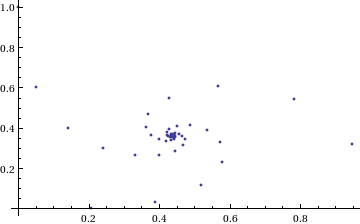
Who would have thought you could get a spiral from power towers? Very nice! So the next question is ‘What would happen if I took a different complex number as my starting point?’ For example – would power towers of (0.5 + i) converge?’

The answer turns out to be yes – power towers of (0.5 + I) converge to 0.541199+ 0.40681 I but the resulting spiral looks rather different from the one above.

tower[base_, size_] := Nest[N[(base^#)] &, base, size];
complexSplit[x_] := {Re[x], Im[x]};
ListPlot[Map[complexSplit, Table[tower[0.5 + I, n], {n, 0, 49, 1}]],
 PlotRange -> All]

The zoo of power tower spirals

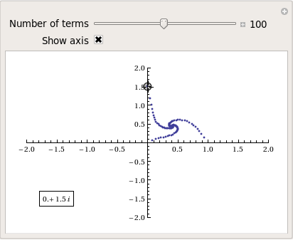
So, taking power towers of two different complex numbers results in two qualitatively different ‘convergence spirals’. I wondered how many different spiral types I might find if I consider the entire complex plane?  I already have all of the machinery I need to perform such an investigation but investigation is much more fun if it is interactive.  Time for a Manipulate

complexSplit[x_] := {Re[x], Im[x]};

tower[base_, size_] := Nest[N[(base^#)] &, base, size];

generatePowerSpiral[p_, nmax_] :=
  Map[complexSplit, Table[tower[p, n], {n, 0, nmax-1, 1}]];

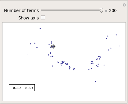
Manipulate[const = p[[1]] + p[[2]] I;
 ListPlot[generatePowerSpiral[const, n],
 PlotRange -> {{-2, 2}, {-2, 2}}, Axes -> ax,
 Epilog -> Inset[Framed[const], {-1.5, -1.5}]], {{n, 100,
 "Number of terms"}, 1, 200, 1,
 Appearance -> "Labeled"}, {{ax, True, "Show axis"}, {True,
 False}}, {{p, {0, 1.5}}, Locator}]

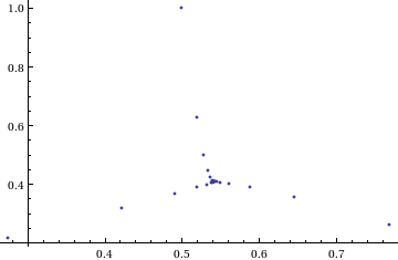
After playing around with this Manipulate for a few seconds it became clear to me that there is quite a rich diversity of these convergence spirals. Here are a couple more

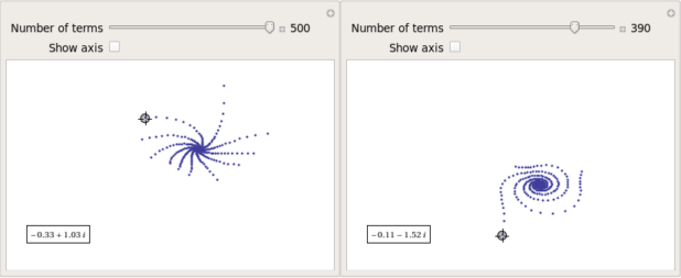
Some of them take a lot longer to converge than others and then there are those that don’t converge at all:

Optimising the code a little

Before I could investigate convergence any further, I had a problem to solve: Sometimes the Manipulate would completely freeze and a message eventually popped up saying “One or more dynamic objects are taking excessively long to finish evaluating……”  What was causing this I wondered?

Well, some values give overflow errors:

In[12]:= generatePowerSpiral[-1 + -0.5 I, 200]

General::ovfl: Overflow occurred in computation. >>
General::ovfl: Overflow occurred in computation. >>
General::ovfl: Overflow occurred in computation. >>
General::stop: Further output of General::ovfl will be suppressed during this calculation. >>

Could errors such as this be making my Manipulate unstable?  Let’s see how long it takes Mathematica to deal with the example above

AbsoluteTiming[ListPlot[generatePowerSpiral[-1  -0.5 I, 200]]]

On my machine, the above command typically takes around 0.08 seconds to complete compared to 0.04 seconds for a tower that converges nicely; it’s slower but not so slow that it should break Manipulate.  Still, let’s fix it anyway.

Look at the sequence of values that make up this problematic power tower

generatePowerSpiral[-0.8 + 0.1 I, 10]

{{-0.8, 0.1}, {-0.668442, -0.570216}, {-2.0495, -6.11826},
{2.47539*10^7,1.59867*10^8}, {2.068155430437682*10^-211800874,
-9.83350984373519*10^-211800875}, {Overflow[], 0}, {Indeterminate,
  Indeterminate}, {Indeterminate, Indeterminate}, {Indeterminate,
  Indeterminate}, {Indeterminate, Indeterminate}}

Everything is just fine until the term {Overflow[],0} is reached; after which we are just wasting time. Recall that the functions I am using to create these sequences are

complexSplit[x_] := {Re[x], Im[x]};
tower[base_, size_] := Nest[N[(base^#)] &, base, size];
generatePowerSpiral[p_, nmax_] :=
  Map[complexSplit, Table[tower[p, n], {n, 0, nmax-1, 1}]];

The first thing I need to do is break out of tower’s Nest function as soon as the result stops being a complex number and the NestWhile function allows me to do this.  So, I could redefine the tower function to be

tower[base_, size_] :=
 NestWhile[N[(base^#)] &, base, MatchQ[#, _Complex] &, 1, size]

However, I can do much better than that since my code so far is massively inefficient.  Say I already have the first n terms of a tower sequence; to get the (n+1)th term all I need to do is a single power operation but my code is starting from the beginning and doing n power operations instead.  So, to get the 5th term, for example, my code does this

I^I^I^I^I

instead of

(4th term)^I

The function I need to turn to is yet another variant of Nest – NestWhileList

fasttowerspiral[base_, size_] :=
 Quiet[Map[complexSplit,
 NestWhileList[N[(base^#)] &, base, MatchQ[#, _Complex] &, 1,
 size, -1]]];

The Quiet function is there to prevent Mathematica from warning me about the Overflow error.  I could probably do better than this and catch the Overflow error coming before it happens but since I’m only mucking around, I’ll leave that to an interested reader.  For now it’s enough for me to know that the code is much faster than before:

(*Original Function*)
AbsoluteTiming[generatePowerSpiral[I, 200];]

{0.036254, Null}

(*Improved Function*)
AbsoluteTiming[fasttowerspiral[I, 200];]

{0.001740, Null}

A factor of 20 will do nicely!

Making Mathematica faster by making it stupid

I’m still not done though. Even with these optimisations, it can take a massive amount of time to compute some of these power tower spirals. For example

spiral = fasttowerspiral[-0.77 - 0.11 I, 100];

takes 10 seconds on my machine which is thousands of times slower than most towers take to compute. What on earth is going on? Let’s look at the first few numbers to see if we can find any clues

In[34]:= spiral[[1 ;; 10]]

Out[34]= {{-0.77, -0.11}, {-0.605189, 0.62837}, {-0.66393,
  7.63862}, {1.05327*10^10,
  7.62636*10^8}, {1.716487392960862*10^-155829929,
  2.965988537183398*10^-155829929}, {1., \
-5.894184073663391*10^-155829929}, {-0.77, -0.11}, {-0.605189,
  0.62837}, {-0.66393, 7.63862}, {1.05327*10^10, 7.62636*10^8}}

The first pair that jumps out at me is {1.71648739296086210^-155829929, 2.96598853718339810^-155829929} which is so close to {0,0} that it’s not even funny! So close, in fact, that they are not even double precision numbers any more. Mathematica has realised that the calculation was going to underflow and so it caught it and returned the result in arbitrary precision.

Arbitrary precision calculations are MUCH slower than double precision ones and this is why this particular calculation takes so long. Mathematica is being very clever but its cleverness is costing me a great deal of time and not adding much to the calculation in this case. I reckon that I want Mathematica to be stupid this time and so I’ll turn off its underflow safety net.

SetSystemOptions["CatchMachineUnderflow" -> False]

Now our problematic calculation takes 0.000842 seconds rather than 10 seconds which is so much faster that it borders on the astonishing. The results seem just fine too!

When do the power towers converge?

We have seen that some towers converge while others do not. Let S be the set of complex numbers which lead to convergent power towers. What might S look like? To determine that I have to come up with a function that answers the question ‘For a given complex number z, does the infinite power tower converge?’ The following is a quick stab at such a function

convergeQ[base_, size_] :=
  If[Length[
     Quiet[NestWhileList[N[(base^#)] &, base, Abs[#1 - #2] > 0.01 &,
       2, size, -1]]] < size, 1, 0];

The tolerance I have chosen, 0.01, might be a little too large but these towers can take ages to converge and I’m more interested in speed than accuracy right now so 0.01 it is. convergeQ returns 1 when the tower seems to converge in at most size steps and 0 otherwise.:

In[3]:= convergeQ[I, 50]
Out[3]= 1

In[4]:= convergeQ[-1 + 2 I, 50]
Out[4]= 0

So, let’s apply this to a section of the complex plane.

towerFract[xmin_, xmax_, ymin_, ymax_, step_] :=
 ArrayPlot[
 Table[convergeQ[x + I y, 50], {y, ymin, ymax, step}, {x, xmin, xmax,step}]]
towerFract[-2, 2, -2, 2, 0.1]

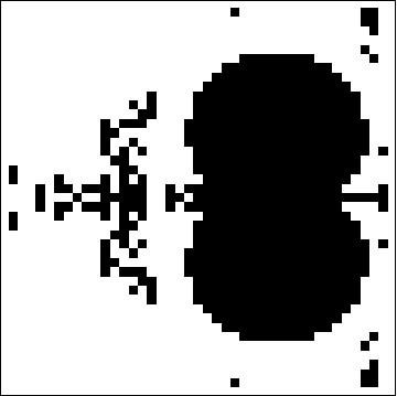
That looks like it might be interesting, possibly even fractal, behaviour but I need to increase the resolution and maybe widen the range to see what’s really going on. That’s going to take quite a bit of calculation time so I need to optimise some more.

Going Parallel

There is no point in having machines with two, four or more processor cores if you only ever use one and so it is time to see if we can get our other cores in on the act.

It turns out that this calculation is an example of a so-called embarrassingly parallel problem and so life is going to be particularly easy for us.  Basically, all we need to do is to give each core its own bit of the complex plane to work on, collect the results at the end and reap the increase in speed. Here’s the full parallel version of the power tower fractal code

(*Complete Parallel version of the power tower fractal code*)

convergeQ[base_, size_] :=
 If[Length[
 Quiet[NestWhileList[N[(base^#)] &, base, Abs[#1 - #2] > 0.01 &,
 2, size, -1]]] < size, 1, 0];

LaunchKernels[];
DistributeDefinitions[convergeQ];
ParallelEvaluate[SetSystemOptions["CatchMachineUnderflow" -> False]];

towerFractParallel[xmin_, xmax_, ymin_, ymax_, step_] :=
 ArrayPlot[
 ParallelTable[
 convergeQ[x + I y, 50], {y, ymin, ymax, step}, {x, xmin, xmax, step}
, Method -> "CoarsestGrained"]]

This code is pretty similar to the single processor version so let’s focus on the parallel modifications.  My convergeQ function is no different to the serial version so nothing new to talk about there.  So, the first new code is

LaunchKernels[];

This launches a set of parallel Mathematica kernels. The amount that actually get launched depends on the number of cores on your machine.  So, on my dual core laptop I get 2 and on my quad core desktop I get 4.

DistributeDefinitions[convergeQ];

All of those parallel kernels are completely clean in that they don’t know about my user defined convergeQ function. This line sends the definition of convergeQ to all of the freshly launched parallel kernels.

ParallelEvaluate[SetSystemOptions["CatchMachineUnderflow" -> False]];

Here we turn off Mathematica’s machine underflow safety net on all of our parallel kernels using the ParallelEvaluate function.

That’s all that is necessary to set up the parallel environment.  All that remains is to change Map to ParallelMap and to add the argument Method -> “CoarsestGrained” which basically says to Mathematica ‘Each sub-calculation will take a tiny amount of time to perform so you may as well send each core lots to do at once’ (click here for a blog post of mine where this is discussed further).

That’s all it took to take this embarrassingly parallel problem from a serial calculation to a parallel one.  Let’s see if it worked.  The test machine for what follows contains a T5800 Intel Core 2 Duo CPU running at 2Ghz on Ubuntu (if you want to repeat these timings then I suggest you read this blog post first or you may find the parallel version going slower than the serial one).  I’ve suppressed the output of the graphic since I only want to time calculation and not rendering time.

(*Serial version*)
In[3]= AbsoluteTiming[towerFract[-2, 2, -2, 2, 0.1];]
Out[3]= {0.672976, Null}

(*Parallel version*)
In[4]= AbsoluteTiming[towerFractParallel[-2, 2, -2, 2, 0.1];]
Out[4]= {0.532504, Null}

In[5]= speedup = 0.672976/0.532504
Out[5]= 1.2638

I was hoping for a bit more than a factor of 1.26 but that’s the way it goes with parallel programming sometimes. The speedup factor gets a bit higher if you increase the size of the problem though. Let’s increase the problem size by a factor of 100.

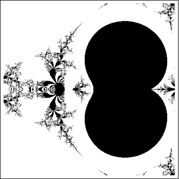
towerFractParallel[-2, 2, -2, 2, 0.01]

The above calculation took 41.99 seconds compared to 63.58 seconds for the serial version resulting in a speedup factor of around 1.5 (or about 34% depending on how you want to look at it).

Other optimisations

I guess if I were really serious about optimising this problem then I could take advantage of the symmetry along the x axis or maybe I could utilise the fact that if one point in a convergence spiral converges then it follows that they all do. Maybe there are more intelligent ways to test for convergence or maybe I’d get a big speed increase from programming in C or F#?  If anyone is interested in having a go at improving any of this and succeeds then let me know.

I’m not going to pursue any of these or any other optimisations, however, since the above exploration is what I achieved in a single train journey to work (The write-up took rather longer though). I didn’t know where I was going and I only worried about optimisation when I had to. At each step of the way the code was fast enough to ensure that I could interact with the problem at hand.

Being mostly ‘fast enough’ with minimal programming effort is one of the reasons I like playing with Mathematica when doing explorations such as this.

Treading where people have gone before

So, back to the power tower story. As I mentioned earlier, I did most of the above in a single train journey and I didn’t have access to the internet. I was quite excited that I had found a fractal from such a relatively simple system and very much felt like I had discovered something for myself. Would this lead to something that was publishable I wondered?

Sadly not!

It turns out that power towers have been thoroughly investigated and the act of forming a tower is called tetration. I learned that when a tower converges there is an analytical formula that gives what it will converge to:

Where W is the Lambert W function (click here for a cool poster for this function).  I discovered that other people had already made Wolfram Demonstrations for power towers too

• The Repeated Power function
• Convergence of a Hyperpower Sequence

There is even a website called tetration.org that shows ‘my’ fractal in glorious technicolor.  Nothing new under the sun eh?

Parting shots

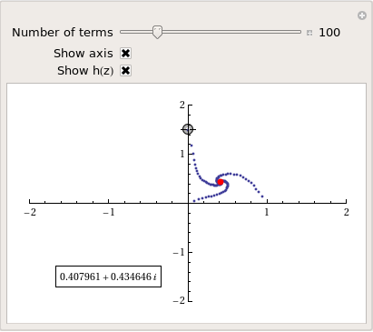
Well, I didn’t discover anything new but I had a bit of fun along the way. Here’s the final Manipulate I came up with

Manipulate[const = p[[1]] + p[[2]] I;
 If[hz,
  ListPlot[fasttowerspiral[const, n], PlotRange -> {{-2, 2}, {-2, 2}},
    Axes -> ax,
   Epilog -> {{PointSize[Large], Red,
      Point[complexSplit[N[h[const]]]]}, {Inset[
       Framed[N[h[const]]], {-1, -1.5}]}}]
  , ListPlot[fasttowerspiral[const, n],
   PlotRange -> {{-2, 2}, {-2, 2}}, Axes -> ax]
  ]
 , {{n, 100, "Number of terms"}, 1, 500, 1, Appearance -> "Labeled"}
 , {{ax, True, "Show axis"}, {True, False}}
 , {{hz, True, "Show h(z)"}, {True, False}}
 , {{p, {0, 1.5}}, Locator}
 , Initialization :> (
   SetSystemOptions["CatchMachineUnderflow" -> False];
   complexSplit[x_] := {Re[x], Im[x]};
   fasttowerspiral[base_, size_] :=
    Quiet[Map[complexSplit,
      NestWhileList[N[(base^#)] &, base, MatchQ[#, _Complex] &, 1,
       size, -1]]];
   h[z_] := -ProductLog[-Log[z]]/Log[z];
   )
 ]

and here’s a video of a zoom into the tetration fractal that I made using spare cycles on Manchester University’s condor pool.

If you liked this blog post then you may also enjoy:

• Simulating Harmonographs
• Polygonal numbers on quadratic number spirals
• The Unreasonable ineffectiveness of factoring
• Quadraflakes, Pentaflakes, Hexaflakes and more
• The equation that says Hi

Lots of people are hitting Walking Randomly looking for info about Mathematica 8 and have had to walk away disappointed….until now!

I’ve been part of the Mathematica 8 beta program for a while now and in order to access the goodies I had to sign an NDA which can be roughly summed up as ‘The first rule of Mathematica 8 beta is that you don’t talk about Mathematica 8 beta.’

As of today, however, I am allowed to show you a tiny little bit of it in advance of it being released. Mathematica 8 will include a massive amount of support for control theory. Here’s a brief preview

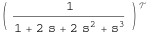
Let’s start by building a transfer function model

myTF = TransferFunctionModel[1/(1 + 2 s + 2 s^2 + s^3), s]

I can find its poles exactly

TransferFunctionPoles[myTF]

{{{-1, -(-1)^(1/3), (-1)^(2/3)}}}

and, of course, numerically

TransferFunctionPoles[myTF] //N

{{{-1., -0.5 - 0.866025 I, -0.5 + 0.866025 I}}}

Here’s its bode plot

BodePlot[myTF]

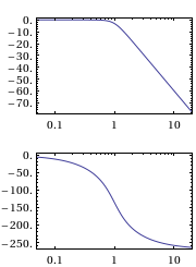
Here’s its response to a unit step function

stepresponse = OutputResponse[myTF, UnitStep[t], t]

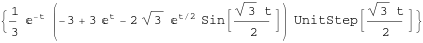
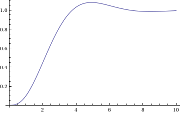
Let’s plot that response

Plot[stepresponse, {t, 0, 10}]

Finally, I convert it to a state space model.

StateSpaceModel[myTF]

That’s the tip of a very big iceberg ;)

Update: Mathematica 8 has now been released.  See https://www.walkingrandomly.com/?p=3018 for more details.

Other Mathematica 8 previews

• The Owen’s T function
• Symbolics and Numerics combine to form new integration Algorithm
• Mathematica, CUDA and GPUs
• Real time image capturing
• 5 new plot commands in Mathematica 8

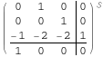
I work at The University of Manchester in the UK and, as some of you may have heard, two of our Professors recently won the Nobel Prize in physics for their discovery of graphene.  Naturally, I wanted to learn more about graphene and, as a fan of Mathematica, I turned to the Wolfram Demonstrations Project to see what I could see.  Click on the images to go to the relevant demonstration.

Back when I used to do physics research myself, I was interested in band structure and it turns out that there is a great demonstration from Vladimir Gavryushin that will help you learn all about the band structure of graphene using the tight binding approximation.

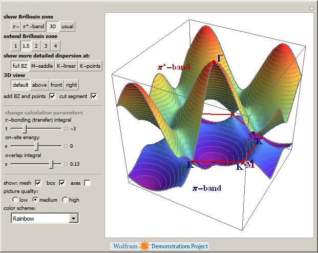
The electronic band structure of a material is important because it helps us to understand (and maybe even engineer) its electronic and optical properties and if you want to know more about its optical properties then the next demonstration from Jessica Alfonsi is for you.

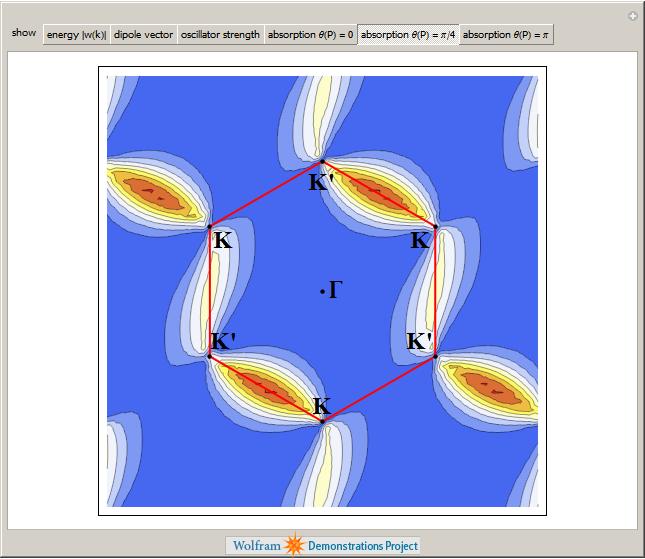
Another professor at Manchester, Niels Walet, produced the next demonstration which asks “Is there a Klein Paradox in Graphene?”

Finally, Graphene can be rolled up to make Carbon Nanotubes as demonstrated by Sándor Kabai.

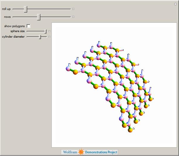
This is just a taster of the Graphene related demonstrations available at The Wolfram Demonstrations project (There are 11 at the time of writing) and I have no doubt that there will be more in the future. Many of them are exceptionally well written and they include lists of references, full source code and, best of all, they can be run for free using the Mathematica Player.

Don’t just read about cutting-edge research, get in there and interact with it!