Walking Randomly

After writing my recent article on GPU accelerated Matrix-Matrix multiplication using Maple, I thought that I’d try the same thing in Mathematica.  However, I instantly hit a problem on my 64bit Windows 7 machine running version 8.0.1 of Mathematica.

In[1]:= a = RandomReal[1, {2, 2}]
Out[1]= {{0.363441, 0.528656}, {0.208881, 0.510232}}

In[2]:= b = RandomReal[1, {2, 2}]
Out[2]= {{0.33536, 0.77615}, {0.537533, 0.788522}}

In[3]:= Dot[a, b]
Out[3]= {{0.406054, 0.698942}, {0.344317, 0.564452}}

In[4]:= Needs["CUDALink`"]
CUDADot[a, b]
Out[5]= {{0.741414, 1.47509}, {0.881849, 1.35297}}

In short, CUDADot gives the wrong result for floating point numbers (on my machine at least).  An upgrade to version 8.0.4 fixed the problem

The Wolfram blog has just published an article previewing the .cdf player on iPad.  I’ve discussed .cdf technology several times before (see Interactive Slinky Thing and Interactive Mathematics in the Web Browser for example) and it forms the basis of the superb Wolfram Demonstrations Project.

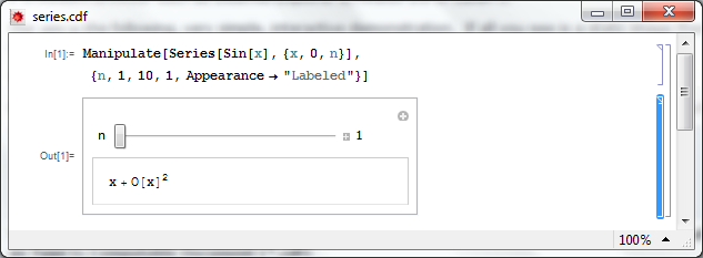
In a nutshell, it is trivially easy to write interactive mathematical applets using Mathematica and publish them to .cdf format.  The magic happens via the Manipulate command which has been around since version 6.  For example, here is the full source code for a simple interactive applet that calculates and displays the power series for sin(x)

Manipulate[
 Series[Sin[x], {x, 0, n}]
 , {n, 1, 10, 1, Appearance -> "Labeled"}
 ]

Here is the result

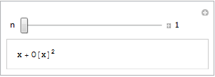
If you have Mathematica 8 or the free .cdf player installed with browser plug-in enabled then you’ll see a fully interactive applet above. Otherwise, you just get a simple image.

Bear in mind that this isn’t showing you a set of pre-computed solutions, it’s actually performing the calculations in real time using the full Mathematica kernel.  With this new player you’ll be able to do that on iPad as well as on your PC. That’s right…Wolfram have taken the full Mathematica kernel and got it running on iPad! It’s not shipping yet but it looks like it’s going to be awesome.

Just imagine…all 7000+ Wolfram Demonstrations on iPad, not to mention your own bespoke code.

There is a preview of the new technology in the video below.

Other articles on mobile mathematics from WalkingRandomly

• Breaking news: Maple Player for Ipad
• MATLAB Mobile brings MATLAB to the iPhone and iPad (sort of)
• Addi – A MATLAB clone for Android phones and tablets
• Math on the iPad #1

My attention was recently drawn to a Google+ post by JerWei Zhang where he evaluates 2^3^4 in various packages and notes that they don’t always agree.  For example, in MATLAB 2010a we have 2^3^4 = 4096 which is equivalent to putting (2^3)^4 whereas Mathematica 8 gives 2^3^4 = 2417851639229258349412352 which is the same as putting 2^(3^4).  JerWei’s post gives many more examples including Excel, Python and Google and the result is always one of these two (although to varying degrees of precision).

What surprised me was the fact that they disagreed at all since I thought that the operator precendence rules were an agreed standard across all software packages.  In this case I’d always use brackets since _I_ am not sure what the correct interpretation of 2^3^4 should be but I would have taken it for granted that there is a standard somewhere and that all of the big hitters in the numerical world would adhere to it.

Looks like I was wrong!

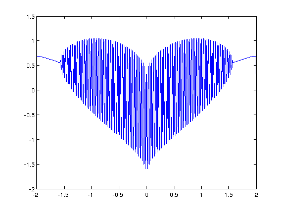
I’ve seen several equations that plot a heart shape over the years but a recent google+ post by Lionel Favre introduced me to a new one.  I liked it so much that I didn’t want to wait until Valentine’s day to share it.  In Mathematica:

Plot[Sqrt[Cos[x]]*Cos[200*x] + Sqrt[Abs[x]] - 0.7*(4 - x*x)^0.01, {x, -2, 2}]

and in MATLAB:

>> x=[-2:.001:2];
>> y=(sqrt(cos(x)).*cos(200*x)+sqrt(abs(x))-0.7).*(4-x.*x).^0.01;
>> plot(x,y)
Warning: Imaginary parts of complex X and/or Y arguments ignored

The result from the MATLAB version is shown below

Update

Rene Grothmann has looked at this equation in a little more depth and plotted it using Euler.

Similar posts

• A little mathematics for Valentine’s day
• The equation that says Hi

Consider this indefinite integral

Feed it to MATLAB’s symbolic toolbox:

int(1/sqrt(x*(2 - x)))

ans =
asin(x - 1)

Feed it to Mathematica 8.0.1:

Integrate[1/Sqrt[x (2 - x)], x] // InputForm

(2*Sqrt[-2 + x]*Sqrt[x]*Log[Sqrt[-2 + x] + Sqrt[x]])/Sqrt[-((-2 + x)*x)]

Let x=1.2 in both results:

MATLAB's answer evaluates to 0.2014
Mathematica's answer evaluates to -1.36944 + 0.693147 I

Discuss!

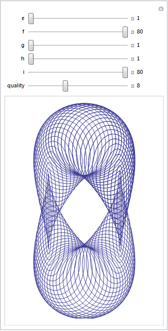
Over at Playing with Mathematica, Sol Lederman has been looking at pretty parametric and polar plots.  One of them really stood out for me, the one that Sol called ‘Slinky Thing’ which could be generated with the following Mathematica command.

ParametricPlot[{Cos[t] - Cos[80 t] Sin[t], 2 Sin[t] - Sin[80 t]}, {t, 0, 8}]

Out of curiosity I parametrised some of the terms and wrapped the whole thing in a Manipulate to see what I could see. I added 5 controllable parameters by turning Sol’s equations into

{Cos[e t] - Cos[f t] Sin[g t], 2 Sin[h t] - Sin[i t]}, {t, 0, 8}

Each parameter has its own slider (below). If you have Mathematica 8, or the free cdf player, installed then the image below will turn into an interactive applet which you can use to explore the parameter space of these equations.

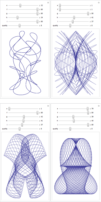
Here are four of my favourites.  If you come up with one that you particularly like then feel free to let me know what the parameters are in the comments.

Over at Sol Lederman’s fantastic new blog, Playing with Mathematica, he shared some code that produced the following figure.

Here’s Sol’s code with an AbsoluteTiming command thrown in.

f[x_, y_] := Module[{},
  If[
   Sin[Min[x*Sin[y], y*Sin[x]]] >
    Cos[Max[x*Cos[y],
       y*Cos[x]]] + (((2 (x - y)^2 + (x + y - 6)^2)/40)^3)/
      6400000 + (12 - x - y)/30, 1, 0]
  ]

 AbsoluteTiming[
\[Delta] = 0.02;
range = 11;
xyPoints = Table[{x, y}, {y, 0, range, \[Delta]}, {x, 0, range, \[Delta]}];
image = Map[f @@ # &, xyPoints, {2}];
]
Rotate[ArrayPlot[image, ColorRules -> {0 -> White, 1 -> Black}], 135 Degree]

This took 8.02 seconds on the laptop I am currently working on (Windows 7 AMD Phenom II N620 Dual core at 2.8Ghz). Note that I am only measuring how long the calculation itself took and am ignoring the time taken to render the image and define the function.

Compiled functions make Mathematica code go faster

Mathematica has a Compile function which does exactly what you’d expect…it produces a compiled version of the function you give it (if it can!). Sol’s function gave it no problems at all.

f = Compile[{{x, _Real}, {y, _Real}}, If[
    Sin[Min[x*Sin[y], y*Sin[x]]] >
     Cos[Max[x*Cos[y],
        y*Cos[x]]] + (((2 (x - y)^2 + (x + y - 6)^2)/40)^3)/
       6400000 + (12 - x - y)/30, 1, 0]
   ];

AbsoluteTiming[
 \[Delta] = 0.02;
 range = 11;
 xyPoints =
  Table[{x, y}, {y, 0, range, \[Delta]}, {x, 0, range, \[Delta]}];
 image = Map[f @@ # &, xyPoints, {2}];
 ]
Rotate[ArrayPlot[image, ColorRules -> {0 -> White, 1 -> Black}],
 135 Degree]

This simple change takes computation time down from 8.02 seconds to 1.23 seconds which is a 6.5 times speed up for hardly any extra coding work. Not too shabby!

Switch to C code to get it even faster

I’m not done yet though! By default the Compile command produces code for the so-called Mathematica Virtual Machine but recent versions of Mathematica allow us to go even further.

Install Visual Studio Express 2010 (and the Windows 7.1 SDK if you are running 64bit Windows) and you can ask Mathematica to convert the function to low level C code, compile it and produce a function object linked to the resulting compiled code. Sounds complicated but is a snap to actually do. Just add

CompilationTarget -> "C"

to the Compile command.

f = Compile[{{x, _Real}, {y, _Real}},
   If[Sin[Min[x*Sin[y], y*Sin[x]]] >
     Cos[Max[x*Cos[y],
        y*Cos[x]]] + (((2 (x - y)^2 + (x + y - 6)^2)/40)^3)/
       6400000 + (12 - x - y)/30, 1, 0]
   , CompilationTarget -> "C"
   ];

AbsoluteTiming[\[Delta] = 0.02;
 range = 11;
 xyPoints =
  Table[{x, y}, {y, 0, range, \[Delta]}, {x, 0, range, \[Delta]}];
 image = Map[f @@ # &, xyPoints, {2}];]
Rotate[ArrayPlot[image, ColorRules -> {0 -> White, 1 -> Black}],
 135 Degree]

On my machine this takes calculation time down to 0.89 seconds which is 9 times faster than the original.

Making the compiled function listable

The current compiled function takes just one x,y pair and returns a result.

In[8]:= f[1, 2]

Out[8]= 1

It can’t directly accept a list of x values and a list of y values. For example for the two points (1,2) and (10,20) I’d like to be able to do f[{1, 10}, {2, 20}] and get the results {1,1}. However what I end up with is an error

f[{1, 10}, {2, 20}]

CompiledFunction::cfsa: Argument {1,10} at position 1 should be a machine-size real number. >>

To fix this I need to make my compiled function listable which is as easy as adding

RuntimeAttributes -> {Listable}

to the function definition.

f = Compile[{{x, _Real}, {y, _Real}},
   If[Sin[Min[x*Sin[y], y*Sin[x]]] >
     Cos[Max[x*Cos[y],
        y*Cos[x]]] + (((2 (x - y)^2 + (x + y - 6)^2)/40)^3)/
       6400000 + (12 - x - y)/30, 1, 0]
   , CompilationTarget -> "C", RuntimeAttributes -> {Listable}
   ];

So now I can pass the entire array to this compiled function at once. No need for Map.

AbsoluteTiming[
 \[Delta] = 0.02;
 range = 11;
 xpoints = Table[x, {x, 0, range, \[Delta]}, {y, 0, range, \[Delta]}];
 ypoints = Table[y, {x, 0, range, \[Delta]}, {y, 0, range, \[Delta]}];
 image = f[xpoints, ypoints];
 ]
Rotate[ArrayPlot[image, ColorRules -> {0 -> White, 1 -> Black}],
 135 Degree]

On my machine this gets calculation time down to 0.28 seconds, a whopping 28.5 times faster than the original. Rendering time is becoming much more of an issue than calculation time in fact!

Parallel anyone?

Simply by adding

Parallelization -> True

to the Compile command I can parallelise the code using threads. Since I have a dual core machine, this might be a good thing to do. Let’s take a look

f = Compile[{{x, _Real}, {y, _Real}},
   If[
    Sin[Min[x*Sin[y], y*Sin[x]]] >
     Cos[Max[x*Cos[y],
        y*Cos[x]]] + (((2 (x - y)^2 + (x + y - 6)^2)/40)^3)/
       6400000 + (12 - x - y)/30, 1, 0]
   , RuntimeAttributes -> {Listable}, CompilationTarget -> "C",
   Parallelization -> True];

AbsoluteTiming[
 \[Delta] = 0.02;
 range = 11;
 xpoints = Table[x, {x, 0, range, \[Delta]}, {y, 0, range, \[Delta]}];
 ypoints = Table[y, {x, 0, range, \[Delta]}, {y, 0, range, \[Delta]}];
 image = f[xpoints, ypoints];
 ]
Rotate[ArrayPlot[image, ColorRules -> {0 -> White, 1 -> Black}],
 135 Degree]

The first time I ran this it was SLOWER than the non-threaded version coming in at 0.33 seconds. Subsequent runs varied and occasionally got as low as 0.244 seconds which is only a few hundredths of a second faster than the original.

If I make the problem bigger, however, by decreasing the size of Delta then we start to see the benefit of parallelisation.

AbsoluteTiming[
 \[Delta] = 0.01;
 range = 11;
 xpoints = Table[x, {x, 0, range, \[Delta]}, {y, 0, range, \[Delta]}];
 ypoints = Table[y, {x, 0, range, \[Delta]}, {y, 0, range, \[Delta]}];
 image = f[xpoints, ypoints];
 ]
Rotate[ArrayPlot[image, ColorRules -> {0 -> White, 1 -> Black}],
 135 Degree]

The above calculation (sans rendering) took 0.988 seconds using a parallelised version of f and 1.24 seconds using a serial version. Rendering took significantly longer! As a comparison lets put a Delta of 0.01 in the original code:

f[x_, y_] := Module[{},
  If[
   Sin[Min[x*Sin[y], y*Sin[x]]] >
    Cos[Max[x*Cos[y],
       y*Cos[x]]] + (((2 (x - y)^2 + (x + y - 6)^2)/40)^3)/
      6400000 + (12 - x - y)/30, 1, 0]
  ]

 AbsoluteTiming[
\[Delta] = 0.01;
range = 11;
xyPoints = Table[{x, y}, {y, 0, range, \[Delta]}, {x, 0, range, \[Delta]}];
image = Map[f @@ # &, xyPoints, {2}];
]
Rotate[ArrayPlot[image, ColorRules -> {0 -> White, 1 -> Black}], 135 Degree]

The calculation time (again, ignoring rendering time) took 32.56 seconds and so our C-compiled, parallel version is almost 33 times faster!

Summary

• The Compile function can make your code run significantly faster by compiling it for the Mathematica Virtual Machine (MVM).  Note that not every function is suitable for compilation.
• If you have a C-compiler installed on your machine then you can switch from the MVM to compiled C-code using a single option statement.  The resulting code is even faster
• Making your functions listable can increase performance.
• Parallelising your compiled function is easy and can lead to even more speed but only if your problem is of a suitable size.
• Sol Lederman has a very cool Mathematica blog – check it out!  The code that inspired this blog post originated there.

Updated January 4th 2011

It is becoming increasingly common for programmers to make use of GPUs (Graphical Processing Units) to speed up their programs substantially.  There are three major low-level programming libraries that allow you to do this in languages such as C; namely CUDA, OpenCL and Microsoft DirectCompute.  Of these three, CUDA is the most developed but it only works on Nvidia graphics cards.

I am often asked if the major commercial math packages support GPU computing and I find myself writing the same summary email over and over again.  So, here is a very brief breakdown of what is currently on offer.  I plan to expand the information contained in this page over time so if you have any information about GPU computing in these packages then let me know.

MATLAB

Core MATLAB contains no support for GPU computing but several organizations (including The Mathworks themselves) have produced add-on toolboxes that add such support:

• Jacket – This is a product from a company called AccelerEyes and is possibly the most advanced and well developed GPU solution for MATLAB currently available.  As of version 2.0 it supports both OpenCL and CUDA frameworks.
• The Mathworks’ Parallel Computing Toolbox (PCT) – If you want to do your MATLAB GPU computing the officially supported way then this is the product you need.  As a bonus, it also allows you to make better use of the multicore processor that almost certainly resides in your machine.  Like many of the offerings on this page, only the CUDA framework is supported so you are out of luck if you don’t have an NVidia graphics card.  Even if you do have an NVidia graphics card then you still might be out of luck since the PCT only supports cards that have compute level 1.3 or above (i.e. double precision only).
• CULA is a set of GPU-accelerated linear algebra libraries utilizing the NVIDIA CUDA parallel computing architecture and it has a MATLAB interface.
• GPUmat – This product is completely free but is less developed than the commercial offerings above.  Again. it is CUDA only
• OpenCL toolbox – The only OpenCL solution for MATLAB I could find.  It is free but development seems to have stalled.

Mathematica

Mathematica 8 has support for both CUDA and OpenCL built in so no need for any add-ons.  Furthermore, it supports both single and double precision GPUs so you can experiment with GPU computing on older, cheaper cards.

Maple

Maple has had some CUDA-only GPU support since version 14.  On the face of it, the CUDA package only appears to contain one accelerated function–Matrix-Matrix multiplication– but when you load this function it accelerates many functions that use matrix-matrix multiply internally.  I’ve never found a definitive list of such functions though.

Mathcad

Mathcad 15 and Mathcad Prime have no support for GPU enhanced computing.

Last month I published an article that included an interactive mathematical demonstration powered by Wolfram’s new CDF (Computable Document Format) player.  These demonstrations work on many modern web-browsers including Internet Explorer 8 and Firefox 3.6.  So, how do you go about adding them to your own websites?

What you need

• Mathematica 8.0.1 or above to create demonstrations.  Viewers of your demonstration only need the free CDF player for their platform.
• A modern browser such as Internet Explorer 8, Firefox 3.6 or Safari 5.
• Basic knowledge of HTML, uploading files to a webserver etc. If you maintain a blog or similar then you almost certainly know enough

Our aim is the following, very simple, interactive demonstration.

If all you see is a static image then you do not have the CDF player or Mathematica 8 correctly installed. Alternatively, you are using an unsupported platform such as Linux, iOS or Android.

Step 1 – Create the .cdf file

Fire up Mathematica, type in and evaluate the following code.  You should get an applet similar to the one above.

Manipulate[
 Series[Sin[x], {x, 0, n}]
 , {n, 1, 10, 1, Appearance -> "Labeled"}
 ]

Save it as a .cdf file called series.cdf by clicking on File->Save as  — Give it the File Name series.cdf and change the Save as Type to Computable Document (*.cdf)

Step 2 – Get a static screenshot

Not everyone is going to have either Mathematica 8 or the free CDF player installed when they visit your website so we need to give them something to look at.  So, lets give them a static image of the Manipulate applet.  As a bonus, this will act as a place holder for the interactive version for those who do have the requisite software.

Open series.cdf in Mathematica and left click on the bracket surrounding the manipulate (see below). Click on Cell->Convert To->Bitmap. Then click on File->Save Selection As . Make sure you change .pdf to something more sensible such as .png

Don’t save your .cdf file at this point or it won’t be interactive. Re-evaluate the code again to get back your interactive Manipulate.

Here’s one I made earlier – series.png

Step 4 – Hide the source code

In this particular instance, I don’t want the user to see the source code.  So, lets sort that out.

• Open series.cdf in Mathematica if you haven’t already and make sure that the Manipulate is evaluated.
• Left click on the inner cell bracket surrounding the Manipulate source code only and click on Cell->Cell Properties and un-tick Open

Step 5 – Hide the cell brackets

Those blue brackets at the far right of the Mathematica notebook are called the Cell brackets and I don’t want to see them on my web site as they make the applet look messy.

• Open series.cdf in Mathematica if you haven’t already
• Open the option inspector: Edit->Preferences->Advanced->Open Option Inspector
• Ensure Show option values is set to “series.cdf” and that they are sorted by category. Click on Apply.
• Click on Cell Options-> Display options and in the right hand pane set ShowCellBracket to False
• Click Apply

Before you save series.cdf ensure that the applet is interactive and not a static bitmap.  If it isn’t interactive then click on Evaluation->Evaluate notebook to re-evaluate the (now hidden) source code.  Also ensure that there is nothing but the applet anywhere else in the notebook.

Step 6 – Get interactive on your website

Upload series.png and series.cdf to your server.  The next thing we need to do is get the static image into our webpage. Here’s what the HTML might look like

<img id="Series_applet" src="series.png" alt="Series demo" />

Obviously, you’ll need to put the full path to series.png on your server in this piece of code. The only thing that is different to the way you might usually use the img tag is that it includes an id; in this case it is Series_applet. We’ll make use of this later.

The magic happens thanks to a small javascript applet called the CDF javascript plugin. Version one is at http://www.wolfram.com/cdf-player/plugin/v1.0/cdfplugin.js and that’s the one I’ll be using here. Here’s the code which needs to be placed before the img tag in your HTML file.

<script src="http://www.wolfram.com/cdf-player/plugin/v1.0/cdfplugin.js"
type="text/javascript"></script><script type="text/javascript">// <![CDATA[
var cdf = new cdf_plugin();
cdf.addCDFObject("Series_applet", "series.cdf", 403,109);
// ]]></script>

The only line you’ll need to change if you use this for anything else is

cdf.addCDFObject("Series_applet", "series.cdf", 403,109);

where Series_applet is the id of the image we wish to replace and series.cdf is the cdf file we want to replace it with. The numbers 403,109 are the dimensions of the applet.  These will not be the same as the .png file as the dimensions of the .cdf file are slightly larger.  I used trial and error to determine what they should be as I haven’t come up with a better way yet (suggestions welcomed).

So that’s it for now. Hope this mini-tutorial was useful. Let me know if you upload any demonstrations to your own website or if you have any comments, questions or problems.

Update (6th June 2011)

Thanks to ‘Paul’ in the comments section, I have discovered that this mechanism won’t work for .cdf files that Wolfram deem are unsafe.  According to Paul the definition of unsafe is as follows:

Dynamic content is considered unsafe if it:

• uses File operations
• uses interprocess communication via MathLink Mathematica Functions
• uses JLink or NETLink
• uses Low-Level Notebook Programming
• uses data as code by Converting between Expressions and Strings
• uses Namespace Management
• uses Options Management
• uses External Programs

I have been a huge fan of the Wolfram Demonstrations project ever since it was launched and have even contributed a few simple demonstrations myself. The project contains thousands of fully interactive mathematical demonstrations that anyone can play with using Wolfram’s free player software and it’s just got a whole lot better.

Now, you can interact with these demonstrations right from the web-browser!

Take the image below, for example. If you don’t have a copy of Wolfram’s new cdf (computable document format) player installed then you’ll just see a static image. Install the player (or Mathematica 8 and the browser-plug in), however, and this image will turn into a fully interactive example.

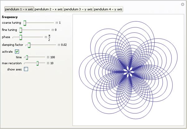
At the moment the browser plug-in only works on Windows and Macintosh but hopefully a Linux version will be on the way soon. Stay tuned to WalkingRandomly for in-depth tutorials on how to go from Mathematica code to fully interactive mathematics in your browser.  The results can be incorporated into the Wolfram Demonstrations project or embedded in your own website like I’ve done here.

Links

• Simulating Harmonographs – Wondering what the above demo is based on?  Find out here.
•  Wolfram Demonstrations Project – Freshly re-designed as of 8th March 2011
• CDF Player – Download Wolfram’s new (and free) Computable Document Format (CDF) player