
Archive for the ‘mathematica’ Category
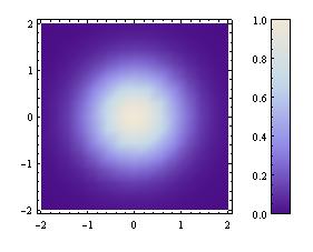
Imagine that you have a function of the form z=f(x,y) and you want to plot it. The result you have in mind is something like this:

The above plot was produced by Matlab and the scale on the right hand side is produced via the colorbar function. I was recently asked if it is possible to easily produce such a scale using Mathematica and after a long search through the documentation the answer was no! Just to make sure that I hadn’t missed something I made a post to comp.soft-sys.mathematica to see what the Mathematica gurus there would make of the problem.
Sure enough there is no simple alternative to colorbar in Mathematica but some helpful soul posted a piece of code that reproduced a similar effect. With a bit of work this turned out to be sufficient for the needs of the person who originally approached me and everyone was happy.
A few days later I discovered that someone called Will Robertson had been following the same thread on the newsgroup and he had used the information posted there to produce a package that allowed a Mathematica user to easily produce ‘colorbar plots’ for both DensityPlots and ContourPlots. I hacked his code so that it supported Plot3D as well and emailed it to him. Between us we tidied up the code a little and submitted it to the wolfram library for everyone to download and use for free.
There is an examples file included in the package distribution that shows how to use it in detail but to give you an idea of what you are going to get here is how to plot the function

once you have downloaded and run the package. The command
ColorbarPlot[Exp[-(#1^2 + #2^2)] &, {-2, 2}, {-2, 2}]
produces the following plot
The above plot is a DensityPlot which is the default type but you can change it using the PlotType option:
ColorbarPlot[Exp[-(#1^2 + #2^2)] &, {-2, 2}, {-2, 2},PlotType->ContourPlot]
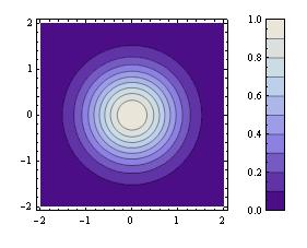
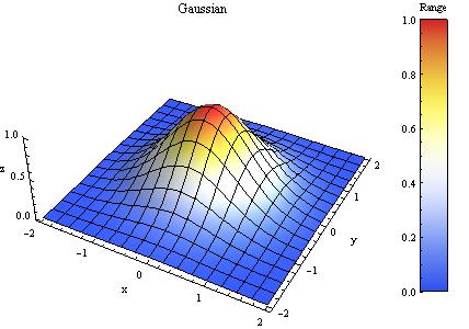
Valid PlotTypes are DensityPlot, ContourPlot and Plot3D but this list will be expanded in future versions. Finally, here is a plot that makes use of lots of options.
f = Exp[-(#1^2 + #2^2)] &
plot = ColorbarPlot[f, {-2, 2}, {-2, 2},
PlotType -> Plot3D,
XLabel -> “x”,
YLabel -> “y”,
ZLabel -> “z”,
Title -> “Gaussian”,
CLabel -> “Range”,
Height -> 300,
Colors -> “TemperatureMap”,
Boxed -> False
]
The package is available for download from here. Comments are welcomed and we hope you like it.
- UPDATE 12th Novermber 2010. Update to version 0.6
- UPDATE 22nd October 2009. Update to version 0.5
- UPDATE 5th June 2008. This package has now been updated to version 0.4
At the moment I am writing an introductory Mathematica course and was recently looking for inspiration for potential exercises. One website I came across (I have lost the link unfortunately) suggested that you get something interesting looking if you plot the following equation over the region -3<x<3, -5<y<5. It also suggested that you should only plot the z values in the range 0<z<0.001.

Suitably intrigued, I issued the required Mathematica commands and got the plot below which spoke to me in a way that no equation ever has before.

So now I have a question – What other messages could one find hidden inside equations like this? For example, is it possible to generate a three letter word with a relatively simple equation such as the one above? Of course if you were allowed to use very complex equations (and make use of Fourier transforms maybe) then I guess you could spell out whatever you choose but that’s no fun.
If anyone finds other such messages in simple(ish) equations then please let me know.
Wolfram’s Mathematica – some people love it, some people loath it – I am definitely one of the former. I have used the package since 2000 when it was at version 4.1 (it’s now at version 6.01) and found it invaluable in the early stages of my PhD. The first time I used it I reproduced around 5 days worth of hand-written symbolic calculations in about 10 minutes – and that included the time it took me to learn how to get Mathematica to do symbolic calculus.
Version 6 of Mathematica came out recently and it was a piece of software I was very excited about (and I don’t often get overly excited about software that isn’t open-source). I had been part of the beta testing program for several months and there was a feature that I had fallen in love with – the ability to make simple but powerful little ‘applets’ using a single command called Manipulate.