
Archive for the ‘programming’ Category
The MATLAB language has become ubiquitous in many fields of applied mathematics such as linear algebra, differential equations, control systems and signal processing among many others. MATLAB is a great tool but it also costs a lot! If you are not a student then MATLAB is a very expensive piece of software. For example, my own academic licensed copy with just 4 toolboxes cost more than the rather high powered laptop I use it on. If I left academia then there would be no chance of me owning a copy unless I found an employer willing to stump up the cash for a commercial license. Commercial licenses cost a LOT more than academic licenses.
Octave – The free alternative
The good news is that there is a free alternative to MATLAB in the form of Octave. Octave attempts to be source compatible with MATLAB which means that, in many cases, your MATLAB code will run as-is on Octave. Many of the undergraduate courses taught at my university (The University of Manchester) could be taught using Octave with little or no modification and I imagine that this would be the case elsewhere. One area where Octave falls down is in the provision of toolboxes but this is improving thanks to the Octave-Forge project.
Addi – The beginnings of MATLAB/Octave on Android
As Dylan said The Times They Are a-Changin’ and there is an ever-increasing segment of world-society that are simply skipping over the PC and going straight to mobile devices for their computing needs. It is possible to get your hands on a functional Android mobile phone or tablet for significantly less than the cost of a PC. These cheap mobile devices may be a lot less powerful than even the cheapest of PCs but they are powerful enough for many purposes and are perfectly capable of outgunning Cray supercomputers from the past.
There is, however, no MATLAB for Android devices. The best we have right now is in the form of Addi, a free Android app that makes use of JMathLib to provide a very scaled-back MATLAB-like experience. Addi is the work of Corbin Champion, an android developer from Portland in the US, and he has much bigger plans for the future.
Full Octave/GNUPlot on Android with no caveats
Corbin is working on a full Octave and GNUPlot* port for Android. He has already included a proof of concept in the latest release of Addi which includes an experimental Octave interpreter. To go from this proof of concept to a fully developed Android port, however, is going to take a lot of work. Corbin is up to the task but he would like our help.
[* – GNUPLot is used as the plotting engine for Octave and includes support for advanced 3D graphics]
Donate as little as $1 to help make this project possible
Corbin has launched a Kickstarter project in order to try to obtain funding for this project. He freely admits that he’ll do the work whether or not it gets funded but will be able to devote much more of his time to the project if the funding request is successful. After all, we all need to eat, even great sotware developers.
Although I have never met him, I believe in Corbin and strongly believe that he will deliver on his promise. So much so that I have pledged $100 to the project out of my own pocket.
If, like me, you want to see a well-developed and supported version of Octave on Android then watch the video below and then head over to Corbin’s kickstarter page to get the full details of his proposal. The minimum donation is only $1 and your money will only be taken if the full funding requirement is met.
Update (16th May 2012): The project (and this post) made it to Slashdot :)
A guest post by Ian Cottam (@iandavidcottam).
I have been a programmer for 40 years this month. I thought I would write a short essay on things I experienced over that time that went into the design of a relatively recent, small program: DropAndCompute. (The purpose and general evolution of that program were described in a blog entry here. Please just watch the video there if you are new to DropAndCompute.)
Once I had the idea for DropAndCompute –inspired equally by the complexity of Condor and the simplicity of Dropbox — I coded and tested it in about two days. (Typically, one bug lasted until it had a real user, but it was no big deal.) My colleague, Mark Whidby, later re-factored/re-coded it to better scale as it grew in popularity here at The University of Manchester. I expect Mark spent about two days on it too. The user interface and basic design did not change. (As the evolution blog discusses, we eventually made the use of Dropbox optional, but that does not detract from this tale.)
Physically dropping programs and their data:
In the early to mid 1970s as well as doing my own programming work I helped scientists in Liverpool to run their code. One approach we used to make them faster was to drop the deck of cards into the input well of a card reader which was remotely connected to the regional supercomputer centre at Manchester. (I never knew what the communication mechanism was – probably a wet string given the technology of the time.) A nearby line printer was similarly connected and our results could be picked up, usually the next day. DropAndCompute is a 21st century version of this activity, without the leg work and humping of large boxes of cards about.
That this approach was worth the effort was made obvious with one of the first card decks I ever submitted. We had been running the code on an ICL 1903A computer in Liverpool; Manchester had a CDC 6600 (hopefully my memory has not let me down – it did become a CDC 7600 at some stage). Running the code locally in Liverpool, with typical data, took around 55 CPU minutes. Dropping it into that card reader so that it automatically ran in Manchester resulted in the jaw dropping time of 4 CPU seconds. (I still had to wait overnight to pick up the results, something that resonates with today’s DropAndCompute users and Manchester’s Condor Pool, which is only large and powerful overnight.)
Capabilities:
Later, but still in the mid 1970s, I worked for Plessey on their System 250 high-reliability, multiprocessor system. It was the first commercial example of a capability architecture. With such there is no supervisor state or privileged code rings or similar. If you held the capability to do something (e.g. read, write or enter another code context) you could do it. If you didn’t hold the appropriate capability, you could not. The only tiny section of code in the System 250 that was special was where capabilities were generated. No one else could make them.
The server side of DropAndCompute generates capabilities to the user client side. They are implemented as zero length files whose information content is just in their names. For job 3159, you get 3159.kill, 3159.vacate and 3159.debug generated*. By dragging and dropping one or more of these zero length files (capabilities) onto the dropbox the remote lower level Condor command code is automatically executed. [* You could try to make your own capability, such as 9513.kill, but it won’t work.]
UNIX and Shell Glue Code:
My initial exposure to the UNIX tools philosophy in the late 1970s profoundly influenced me (and still does). In essence, it says that one should build new software by inventing ‘glue’ to stick existing components together. The UNIX Shell is often the language of choice for this, and was for me. DropAndCompute is a good example of where a little bit of glue produced a hopefully impressive synergy.
The Internet not The Web:
DropAndCompute uses the Internet (clearly). It is not a Web application. I only mention this as some younger programmers, who have grown up with the Web always being there, seem to think the best/only architecture to use for a software system design is one implemented through a web browser using web services. I am grateful to be able to remember pre-Web days, as much as I love what Tim Berners-Lee created for us.
Client-Server:
I’m not sure when I first became aware of client-server architecture. I know a famous computer scientist (the late David Wheeler*) once described it as simply the obvious way to implement software systems. For my part, I’m a believer in the less code the client side (user) needs to install the better (less to go wrong on strange environments one has no control over). In the case of DropAndCompute if the user had Dropbox, it was nothing to install, and just downloading Dropbox if they didn’t.
[* As well as being a co-inventer of the subroutine, David Wheeler led the team that designed the first operational capability-based computer: the Cambridge University CAP.]
Rosetta – Software as Magic:
Around a decade ago I worked for Transitive, a University of Manchester spin-out, and the company that produced Rosetta for Apple. With apologies to Arthur C Clarke: all great software appears to be magic to the user. The simpler the user interface, often the more complex the underlying system is to implement the magic. This is true, for example, for Apple iOS and OS X and for Dropbox (simpler, and yet I would bet that it is internally more complex, than its many competitors). One small part of OS X I helped with is Rosetta (or was, as Apple dropped it from the Lion 10.7 release of OS X). Rosetta dynamically (i.e. on-the-fly) translates PowerPC applications into Intel x86 code. There is no noticeable user interface: you double click your desired application, like any other, and, if needed, Rosetta is invoked to do its job in the background.
I have read many interesting web based discussions about Rosetta, several say, or imply, that it is a relatively simple piece of software: nothing could be further from the truth. It’s likely still a commercial secret how it works, but if it were simple, Apple’s transition to Intel would likely have been a disaster. It took a lot of smart people a long time to make the magic appear that simple.
I tried to keep DropAndCompute’s interface to the user as simple as possible, even where it added some complexity to its implementation. The National Grid Service in the UK did their own version of DropAndCompute, but, for my taste, added too many bells and whistles.
In Conclusion:
I hope this brief essay has been of interest and given some insight into how many years of software/system design experience come to be applied, even to small software systems, both consciously and subconsciously, and always, hopefully, with good taste. Hide complexity, keep it simple for the user, make them think it is simply magic!
Intel have just released their OpenCL Software Development Kit (SDK) for Intel processors. The good news is that this version targets the on-die GPU as well as the CPU allowing truly heterogeneous programming. The bad news is that the GPU goodness is for 3rd Generation ‘Ivy Bridge‘ Processors only– us backward Sandy Bridge users have been left in the cold :(
A quick scan through the release notes reveals the following:-
- OpenCL access to the on-die GPU part is currently for Windows only. Linux users only have CPU support at the moment.
- No access to the GPU part of Sandy Bridge Processors via this implementation.
- The GPU part has single precision only (I guess we’ll see many more mixed-precision algorithms from now on)
I don’t have access to an Ivy Bridge processor and so can’t have a play but I’m looking forward to seeing how much performance OpenCL programmers can squeeze out of this new implementation.
Other WalkingRandomly posts on GPU computing
These days almost all of us are carrying around seriously capable little computers in the form of our mobile phones. Although these devices have a similar amount of horsepower to supercomputers of old, most of us only use a fraction of their potential– after all, you don’t need a supercompter to send text messages, look at pictures of cats or throw birds at pigs. I believe that the only way to fully unlock the true potential of these devices is to program them yourself.
From fully fledged applications to little snippets of code, I think that there’s something enormously satisfying about writing your own computer programs and it doesn’t have to be difficult to do so. The following 9 apps will allow you to write programs for your Android mobile phone in a variety of languages including C, BASIC, Lisp and MATLAB m-code using only your Android phone. Although you’ll not be able to use them to write the next 3D blockbuster game, you will be able to solve some interesting problems, learn a trick or two and have a lot of fun.
C4droid – £0.95
With c4droid you get the ability to write, compile and run C and C++ programs using only your Android device. That’s a lot of functionality for only 95p!
Out of the box C4droid only handles C programs, making use of a modified version of the Tiny C Compiler to do the compilation work. The standard C library is provided by uClibc which is specially designed for use on embedded systems.
In order to run C++ programs you need to additionally install the free GCC plugin for C4droid — something that I personally haven’t done yet due to its large size. One of the most common user-complaints appears to be ‘this app doens’t allow me to use iostream.h’ which essentially demonstrates that the installation instructions were not followed. Since iostream.h is a C++ library, you’ll need to install and configure the GCC plugin to get access to it and full instructions on how to do this are given on c4droid’s Google Play page.
You only get access to the standard C library with C4droid which means that you can’t generate graphical output or interact with the phone’s hardware in any way (bluetooth, accelerometers, that sort of thing) but that doesn’t stop this from being an impressive piece of work. Also, for an extra 95p you can run pascal programs using the Pascal plugin for C4droid.
C4droid is a superb app that will be invaluable for anyone learning C,C++ or Pascal or for those of us that simply like to fiddle about with these languages on the go.
- C4droid on Google Play
- GCC plugin for c4droid (needed for C++ access)
- Pascal plugin for C4droid – provides the ability to compile and run Pascal programs
Mintoris Basic – £3.77
At the risk of showing my age, I’ll tell you that I first learned how to program in BASIC (Beginners All-Purpose Symbolic Instruction Code) on the Sinclair ZX Spectrum and so I will always have a fondness for the language. Mintoris Basic is a very fully featured implementation of the BASIC programming language and is significantly more powerful than the implementation I cut my teeth on back in the day.
As well as having all of the stuff you’d expect in a BASIC implementation (loops, strings, variables, functions, decisions, graphics etc), Mintoris also allows you to interact with some of your phone’s hardware including Bluetooth, battery level, GPS, and various sensors. Furthermore, you can attach your programs to shortcuts and launch them from your home screens. The level of functionality is so high that you can write some rather nifty apps with relatively little effort.
- Get Mintoris Basic from Google Play
- Mintoris Basic official website
- Mintoris Basic Forum
- Mintoris Basic on Facebook
Frink – Free
Frink is a great language developed by Alan Eliasen that has been around since 2001. Named after Professor Frink from The Simpsons, Frink runs on almost every device you can possibly imagine and has some very interesting features including interval arithmetic, tracking of units of measure throughout calculations, arbitrary precision numbers, regular expressions and graphics.
- Get Frink from Google Play
- What’s new – Frink is under very active development. See here for the new stuff
- Many example programs in Frink
- Extensive documentation for Frink
RFO BASIC! + SQL – Free
This implementation of BASIC is completely free and is described as a labour of love by the author, Paul Laughton. Paul is my kind of geek since he is the curator of The Dr. Richard Feynman Observatory and author of Atari Basic and Apple DOS 3.1 among other things.
The feature list of RFO BASIC is impressive and includes Graphics (with Multi-touch), SQL, GPS, Device Sensors, Camera and loads more. There’s a great forum with lots of very engaged developers who are writing some very nice programs.
There are two ways to deploy your programs–either as scripts that require RFO BASIC to be installed or as compiled,standalone programs that can even be added to Google Play (formerly known as the Android Market’).
- RFO BASIC on Google Play
- RFO BASIC Forum
- RFO BASIC website
- De Re BASIC! – The .pdf manual for RFO BASIC
Addi and Mathmatiz – Free
These are two MATLAB clones for Android. I’ve mentioned Addi before and they have both been covered over at Alasdair’s Musings so I won’t go into detail here other than to say that they are very cool! Linear algebra, scripting and plotting on your phone!
tiny Lisp ISLisproid
Lisp is a very old programming language which first saw the light of day in 1958! According to wikipedia, the only langauge older than Lisp that is still in common use is Fortran! With this app you can play with the language of the ancients on your super-modern smartphone. This is a no-frills app..essentially little more than a command line shell and list interpreter but that is perhaps as it should be.
MathStudio – £12.99
I’ve been using MathStudio (formerly SpaceTime Mathematics) for quite a few years now on various operating systems and it’s great to finally have it on Android. MathStudio is a fully featured computer algebra system for your mobile phone– think mini Mathematica or Maple and you are thinking along the right lines. With this app you can write scripts that make use of advanced mathematical features, 2D and 3D graphics, animations and interactive demonstrations.
- MathStudio at GooglePlay
- MathStudio official website
- A set of MathStudio examples and demonstrations
- MathStudio Forum
SigmaScript – Free
SigmaScript is a free implementatuion of the Lua scripting language for Android devices developed by Logimath. You get an editor, scripting engine, small console output and a few simple code examples. No graphics or anything fancy but a very nice way to play with an interesting language.
This article is the third part of a series where I look at rewriting a particular piece of MATLAB code using various techniques. The introduction to the series is here and the introduction to the larger series of GPU articles for MATLAB is here.
Last time I used The Mathwork’s Parallel Computing Toolbox in order to modify a simple correlated asset calculation to run on my laptop’s GPU rather than its CPU. Performance was not as good as I had hoped and I never managed to get my laptop’s GPU (an NVIDIA GT555M) to beat the CPU using functions from the parallel computing toolbox. Transferring the code to a much more powerful Tesla GPU card resulted in a four times speed-up compared to the CPU in my laptop.
This time I’ll take a look at AccelerEyes’ Jacket, a third party GPU solution for MATLAB.
Attempt 1 – Make as few modifications as possible
I started off just as I did for the parallel computing toolbox GPU port; by taking the best CPU-only code from part 1 (optimised_corr2.m) and changing a load of data-types from double to gdouble in order to get the calculation to run on my laptop’s GPU using Jacket v1.8.1 and MATLAB 2010b. I also switched to using the GPU versions of various functions such as grandn instead of randn for example. Functions such as cumprod needed no modifications at all since they are nicely overloaded; if the argument to cumprod is of type double then the calculation happens on the CPU whereas if it is gdouble then it happens on the GPU.
Now, one thing that I don’t like about Jacket’s implementation is that many of the functions return single precision numbers by default. For example, if you do
a=grand(1,10)
then you end up with 10 numbers of type gsingle. To get double precision numbers you have to do
grandn(1,10,'double')
Now you may be thinking ‘what’s the big deal? – it’s just a bit of syntax so get over it’ and I guess that would be a fair comment. Supporting single precision also allows users of legacy GPUs to get in on the GPU-accelerated action which is a good thing. The problem as I see it is that almost everything else in MATLAB uses double precision numbers as the default and so it’s easy to get caught out. I would much rather see functions such as grand return double precision by default with the option to use single precision if required–just like almost every other MATLAB function out there.
The result of my ‘port’ is GPU_jacket_corr1.m
One thing to note in this version, along with all subsequent Jacket versions, is the following command that appears at the very end of the program.
gsync;
This is very important if you want to get meaningful timing results since it ensures that all GPU computations have finished before execution continues. See the Jacket documentation on gysnc and this blog post on timing Jacket code for more details.
The other thing I’ll mention is that, in this version, I do this:
Corr = [1 0.4; 0.4 1];
UpperTriangle=gdouble(chol(Corr));
instead of
Corr = gdouble([1 0.4; 0.4 1]);
UpperTriangle=chol(Corr);
In other words, I do the cholesky decomposition on the CPU and move the results to the GPU rather than doing the calculation on the GPU. This is mainly because I don’t have access to a Jacket DLA license but it’s probably the best thing to do anyway since such a small decomposition probably won’t happen any faster on the GPU.
So, how does it perform. I ran it three times with the now usual parameters of 100000 simulations done in blocks of 125 (see the CPU version for how I came to choose 125)
>> tic;GPU_jacket_corr1;toc
Elapsed time is 40.691888 seconds.
>> tic;GPU_jacket_corr1;toc
Elapsed time is 32.096796 seconds.
>> tic;GPU_jacket_corr1;toc
Elapsed time is 32.039982 seconds.
Just like the Parallel Computing Toolbox, the first run is slower because of GPU warmup overheads. Also, just like the PCT, performance stinks! It’s clearly not enough, in this case at least, to blindly throw in a few gdoubles and hope for the best. It is worth noting, however, that this case is nowhere near as bad as the 900+ seconds we saw in the similar parallel computing toolbox version.
Jacket has punished me for being stupid (or optimistic if you want to be polite to me) but not as much as the PCT did.
Attempt 2 – Convert from a script to a function
When working with the Parallel Computing Toolbox I demonstrated that a switch from a script to a function yielded some speed-up. This wasn’t the case with the Jacket version of the code. The functional version, GPU_jacket_corr2.m, showed no discernable speed improvement compared to the script.
%Warm up run performed previously
>> tic;GPU_jacket_corr2(100000,125);toc
Elapsed time is 32.230638 seconds.
>> tic;GPU_jacket_corr2(100000,125);toc
Elapsed time is 32.179734 seconds.
>> tic;GPU_jacket_corr2(100000,125);toc
Elapsed time is 32.114864 seconds.
Attempt 3 – One big matrix multiply!
The original version of this calculation performs thousands of very small matrix multiplications and last time we saw that switching to a single, large matrix multiplication brought significant speed improvements on the GPU. Modifying the code to do this with Jacket is a very similar process to doing it for the PCT so I’ll omit the details and just present the code, GPU_jacket_corr3.m
%Warm up runs performed previously
>> tic;GPU_jacket_corr3(100000,125);toc
Elapsed time is 2.041111 seconds.
>> tic;GPU_jacket_corr3(100000,125);toc
Elapsed time is 2.025450 seconds.
>> tic;GPU_jacket_corr3(100000,125);toc
Elapsed time is 2.032390 seconds.
Now that’s more like it! Finally we have a GPU version that runs faster than the CPU on my laptop. We can do better, however, since the block size of 125 was chosen especially for my CPU. With this Jacket version bigger is better and we get much more speed-up by switching to a block size of 25000 (I run out of memory on the GPU if I try even bigger block sizes).
%Warm up runs performed previously
>> tic;GPU_jacket_corr3(100000,25000);toc
Elapsed time is 0.749945 seconds.
>> tic;GPU_jacket_corr3(100000,25000);toc
Elapsed time is 0.749333 seconds.
>> tic;GPU_jacket_corr3(100000,25000);toc
Elapsed time is 0.749556 seconds.
Now this is exciting! My laptop GPU with Jacket 1.8.1 is faster than a high-end Tesla card using the parallel computing toolbox for this calculation. My excitement was short lived, however, when I looked at the resulting distribution. The random number generator in Jacket 1.8.1 gave a completely different distribution when compared to generators from other sources (I tried two CPU generators from The Mathworks and one from The Numerical Algorithms Group). The only difference in the code that generated the results below is the random number generator used.
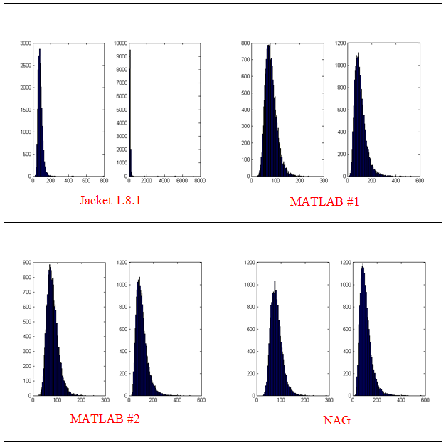
- The results shown in these plots were for only 20,000 simulations rather than the 100,000 I’ve been using elsewhere in this post. I found this bug in the development stage of these posts where I was using a smaller number of simulations.
- Jacket 1.8.1 is using Jackets old grandn function with the ‘double’ option set
- MATLAB #1 is using MATLAB’s randn using the Comb Recursive algorithm on the CPU
- MATLAB #2 is using MATLAB’s randn using the default Mersenne Twister on the CPU
- NAG is using a Wichman-Hill generator
I sent my code to AccelerEye’s customer support who confirmed that this seemed to be a bug in their random number generator (an in-house Mersenne Twister implementation). Less than a week later they offered me a new preview of Jacket from their Nightly builds where the old RNG had been replaced with the Mersenne Twister implementation produced by NVidia and I’m happy to confirm that not only does this fix the results for my code but it goes even faster! Superb customer service!
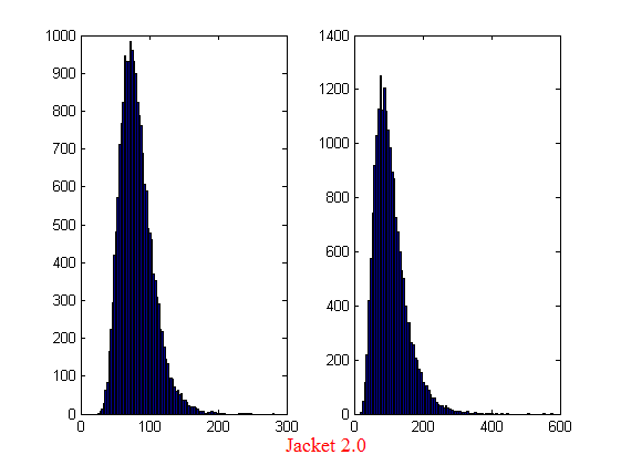
This new RNG is now the default in version 2.0 of Jacket. Here’s the distribution I get for 20,000 simulations (to stay in line with the plots shown above).
Switching back to 100,000 simulations to stay in line with all of the other benchmarks in this series gives the following times on my laptop’s GPU
%Warm up runs performed previously
>> tic;prices=GPU_jacket_corr3(100000,25000);toc
Elapsed time is 0.696891 seconds.
>> tic;prices=GPU_jacket_corr3(100000,25000);toc
Elapsed time is 0.697596 seconds.
>> tic;prices=GPU_jacket_corr3(100000,25000);toc
Elapsed time is 0.697312 seconds.
This is almost 5 times faster than the 3.42 seconds managed by the best CPU version from part 1. I sent my code to AccelerEyes and asked them to run it on a more powerful GPU, a Tesla C2075, and these are the results they sent back
Elapsed time is 5.246249 seconds. %warm up run
Elapsed time is 0.158165 seconds.
Elapsed time is 0.156529 seconds.
Elapsed time is 0.156522 seconds.
Elapsed time is 0.156501 seconds.
So, the Tesla is 4.45 times faster than my laptop’s GPU for this application and a very useful 21.85 times faster than my laptop’s CPU.
Results Summary
- Best CPU Result on laptop (i7-2630GM)with pure MATLAB code – 3.42 seconds
- Best GPU Result with PCT on laptop (GT555M) – 4.04 seconds
- Best GPU Result with PCT on Tesla M2070 – 0.85 seconds
- Best GPU Result with Jacket on laptop (GT555M) – 0.7 seconds
- Best GPU Result with Jacket on Tesla M2075 – 0.16 seconds
Test System Specification
- Laptop model: Dell XPS L702X
- CPU:Intel Core i7-2630QM @2Ghz software overclockable to 2.9Ghz. 4 physical cores but total 8 virtual cores due to Hyperthreading.
- GPU:GeForce GT 555M with 144 CUDA Cores. Graphics clock: 590Mhz. Processor Clock:1180 Mhz. 3072 Mb DDR3 Memeory
- RAM: 8 Gb
- OS: Windows 7 Home Premium 64 bit.
- MATLAB: 2011b
Acknowledgements
Thanks to Yong Woong Lee of the Manchester Business School as well as various employees at AccelerEyes for useful discussions and advice. Any mistakes that remain are all my own.
This article is the second part of a series where I look at rewriting a particular piece of MATLAB code using various techniques. The introduction to the series is here and the introduction to the larger series of GPU articles for MATLAB on WalkingRandomly is here.
Attempt 1 – Make as few modifications as possible
I took my best CPU-only code from last time (optimised_corr2.m) and changed a load of data-types from double to gpuArray in order to get the calculation to run on my laptop’s GPU using the parallel computing toolbox in MATLAB 2010b. I also switched to using the GPU versions of various functions such as parallel.gpu.GPUArray.randn instead of randn for example. Functions such as cumprod needed no modifications at all since they are nicely overloaded; if the argument to cumprod is of type double then the calculation happens on the CPU whereas if it is gpuArray then it happens on the GPU.
The above work took about a minute to do which isn’t bad for a CUDA ‘porting’ effort! The result, which I’ve called GPU_PCT_corr1.m is available for you to download and try out.
How about performance? Let’s do a quick tic and toc using my laptop’s NVIDIA GT 555M GPU.
>> tic;GPU_PCT_corr1;toc
Elapsed time is 950.573743 seconds.
The CPU version of this code took only 3.42 seconds which means that this GPU version is over 277 times slower! Something has gone horribly, horribly wrong!
Attempt 2 – Switch from script to function
In general functions should be faster than scripts in MATLAB because more automatic optimisations are performed on functions. I didn’t see any difference in the CPU version of this code (see optimised_corr3.m from part 1 for a CPU function version) and so left it as a script (partly so I had an excuse to discuss it here if I am honest). This GPU-version, however, benefits noticeably from conversion to a function. To do this, add the following line to the top of GPU_PCT_corr1.m
function [SimulPrices] = GPU_PTC_corr2( n,sub_size)
Next, you need to delete the following two lines
n=100000;                       %Number of simulations
sub_size = 125;
Finally, add the following to the end of our new function
end
That’s pretty much all I did to get GPU_PCT_corr2.m. Let’s see how that performs using the same parameters as our script (100,000 simulations in blocks of 125). I used script_vs_func.m to run both twice after a quick warm-up iteration and the results were:
Warm up
Elapsed time is 1.195806 seconds.
Main event
script
Elapsed time is 950.399920 seconds.
function
Elapsed time is 938.238956 seconds.
script
Elapsed time is 959.420186 seconds.
function
Elapsed time is 939.716443 seconds.
So, switching to a function has saved us a few seconds but performance is still very bad!
Attempt 3 – One big matrix multiply!
So far all I have done is take a program that works OK on a CPU, and run it exactly as-is on the GPU in the hope that something magical would happen to make it go faster. Of course, GPUs and CPUs are very different beasts with differing sets of strengths and weaknesses so it is rather naive to think that this might actually work. What we need to do is to play to the GPUs strengths more and the way to do this is to focus on this piece of code.
for i=1:sub_size
     CorrWiener(:,:,i)=parallel.gpu.GPUArray.randn(T-1,2)*UpperTriangle;
end
Here, we are performing lots of small matrix multiplications and, as mentioned in part 1, we might hope to get better performance by performing just one large matrix multiplication instead. To do this we can change the above code to
%Generate correlated random numbers
%using one big multiplication
randoms = parallel.gpu.GPUArray.randn(sub_size*(T-1),2);
CorrWiener = randoms*UpperTriangle;
CorrWiener = reshape(CorrWiener,(T-1),sub_size,2);
%CorrWiener = permute(CorrWiener,[1 3 2]); %Can't do this on the GPU in 2011b or below

%poor man's permute since GPU permute if not available in 2011b
CorrWiener_final = parallel.gpu.GPUArray.zeros(T-1,2,sub_size);
for s = 1:2
    CorrWiener_final(:, s, :) = CorrWiener(:, :, s);
end
The reshape and permute are necessary to get the matrix in the form needed later on. Sadly, MATLAB 2011b doesn’t support permute on GPUArrays and so I had to use the ‘poor mans permute’ instead.
The result of the above is contained in GPU_PCT_corr3.m so let’s see how that does in a fresh instance of MATLAB.
>> tic;GPU_PCT_corr3(100000,125);toc
Elapsed time is 16.666352 seconds.
>> tic;GPU_PCT_corr3(100000,125);toc
Elapsed time is 8.725997 seconds.
>> tic;GPU_PCT_corr3(100000,125);toc
Elapsed time is 8.778124 seconds.
The first thing to note is that performance is MUCH better so we appear to be on the right track. The next thing to note is that the first evaluation is much slower than all subsequent ones. This is totally expected and is due to various start-up overheads.
Recall that 125 in the above function calls refers to the block size of our monte-carlo simulation. We are doing 100,000 simulations in blocks of 125– a number chosen because I determined empirically that this was the best choice on my CPU. It turns out we are better off using much larger block sizes on the GPU:
>> tic;GPU_PCT_corr3(100000,250);toc
Elapsed time is 6.052939 seconds.
>> tic;GPU_PCT_corr3(100000,500);toc
Elapsed time is 4.916741 seconds.
>> tic;GPU_PCT_corr3(100000,1000);toc
Elapsed time is 4.404133 seconds.
>> tic;GPU_PCT_corr3(100000,2000);toc
Elapsed time is 4.223403 seconds.
>> tic;GPU_PCT_corr3(100000,5000);toc
Elapsed time is 4.069734 seconds.
>> tic;GPU_PCT_corr3(100000,10000);toc
Elapsed time is 4.039446 seconds.
>> tic;GPU_PCT_corr3(100000,20000);toc
Elapsed time is 4.068248 seconds.
>> tic;GPU_PCT_corr3(100000,25000);toc
Elapsed time is 4.099588 seconds.
The above, rather crude, test suggests that block sizes of 10,000 are the best choice on my laptop’s GPU. Sadly, however, it’s STILL slower than the 3.42 seconds I managed on the i7 CPU and represents the best I’ve managed using pure MATLAB code. The profiler tells me that the vast majority of the GPU execution time is spent in the cumprod line and in random number generation (over 40% each).
Trying a better GPU
Of course now that I have code that runs on a GPU I could just throw it at a better GPU and see how that does. I have access to MATLAB 2011b on a Tesla M2070 hooked up to a Linux machine so I ran the code on that. I tried various block sizes and the best time was 0.8489 seconds with the call GPU_PCT_corr3(100000,20000) which is just over 4 times faster than my laptop’s CPU.
Ask the Audience
Can you do better using just the GPU functionality provided in the Parallel Computing Toolbox (so no bespoke CUDA kernels or Jacket just yet)? I’ll be looking at how AccelerEyes’ Jacket myself in the next post.
Results so far
- Best CPU Result on laptop (i7-2630GM)with pure MATLAB code – 3.42 seconds
- Best GPU Result with PCT on laptop (GT555M) – 4.04 seconds
- Best GPU Result with PCT on Tesla M2070 – 0.85 seconds
Test System Specification
- Laptop model: Dell XPS L702X
- CPU: Intel Core i7-2630QM @2Ghz software overclockable to 2.9Ghz. 4 physical cores but total 8 virtual cores due to Hyperthreading.
- GPU: GeForce GT 555M with 144 CUDA Cores. Graphics clock: 590Mhz. Processor Clock:1180 Mhz. 3072 Mb DDR3 Memeory
- RAM: 8 Gb
- OS: Windows 7 Home Premium 64 bit.
- MATLAB: 2011b
Acknowledgements
Thanks to Yong Woong Lee of the Manchester Business School as well as various employees at The Mathworks for useful discussions and advice. Any mistakes that remain are all my own :)
Recently, I’ve been working with members of The Manchester Business School to help optimise their MATLAB code. We’ve had some great successes using techniques such as vectorisation, mex files and The NAG Toolbox for MATLAB (among others) combined with the raw computational power of Manchester’s Condor Pool (which I help run along with providing applications support).
A couple of months ago, I had the idea of taking a standard calculation in computational finance and seeing how fast I could make it run on MATLAB using various techniques. I’d then write these up and publish here for comment.
So, I asked one of my collaborators, Yong Woong Lee, a doctoral researcher in the Manchester Business School, if he could furnish me with a very simple piece computational finance code. I asked for something that was written to make it easy to see the underlying mathematics rather than for speed and he duly obliged with several great examples. I took one of these examples and stripped it down even further to its very bare bones. In doing so I may have made his example close to useless from a computational finance point of view but it gave me something nice and simple to play with.
What I ended up with was a simple piece of code that uses monte carlo techniques to find the distribution of two correlated assets: original_corr.m
%ORIGINAL_CORR - The original, unoptimised code that simulates two correlated assets

%% Correlated asset information
CurrentPrice = [78 102];       %Initial Prices of the two stocks
Corr = [1 0.4; 0.4 1];         %Correlation Matrix
T = 500;                       %Number of days to simulate = 2years = 500days
n = 100000;                    %Number of simulations
dt = 1/250;                    %Time step (1year = 250days)
Div=[0.01 0.01];               %Dividend
Vol=[0.2 0.3];                 %Volatility

%%Market Information
r = 0.03;                      %Risk-free rate

%% Define storages
SimulPriceA=zeros(T,n);    %Simulated Price of Asset A
SimulPriceA(1,:)=CurrentPrice(1);
SimulPriceB=zeros(T,n);    %Simulated Price of Asset B
SimulPriceB(1,:)=CurrentPrice(2);

%% Generating the paths of stock prices by Geometric Brownian Motion
UpperTriangle=chol(Corr);    %UpperTriangle Matrix by Cholesky decomposition

for i=1:n
   Wiener=randn(T-1,2);
   CorrWiener=Wiener*UpperTriangle;
   for j=2:T
      SimulPriceA(j,i)=SimulPriceA(j-1,i)*exp((r-Div(1)-Vol(1)^2/2)*dt+Vol(1)*sqrt(dt)*CorrWiener(j-1,1));
      SimulPriceB(j,i)=SimulPriceB(j-1,i)*exp((r-Div(2)-Vol(2)^2/2)*dt+Vol(2)*sqrt(dt)*CorrWiener(j-1,2));
   end
end

%% Plot the distribution of final prices
% Comment this section out if doing timings
% subplot(1,2,1);hist(SimulPriceA(end,:),100);
% subplot(1,2,2);hist(SimulPriceB(end,:),100);
On my laptop, this code takes 10.82 seconds to run on average. If you comment out the final two lines then it’ll take a little longer and will produce a histogram of the distribution of final prices.
I’m going to take this code and modify it in various ways to see how different techniques and technologies can make it run more quickly. Here is a list of everything I have done so far.
- Standard vectorisation (This article)
- Running on a GPU using the Parallel Computing Toolbox
- Running on a GPU using Jacket from AccelerEyes
Vectorisation – removing loops to make code go faster
Now, the most obvious optimisation that we can do with code like this is to use vectorisation to get rid of that double loop. The cumprod command is the key to doing this and the resulting code looks as follows: optimised_corr1.m
%OPTIMISED_CORR1 - A pure-MATLAB optimised code that simulates two correlated assets

%% Correlated asset information
CurrentPrice = [78 102];       %Initial Prices of the two stocks
Corr = [1 0.4; 0.4 1];         %Correlation Matrix
T = 500;                       %Number of days to simulate = 2years = 500days
Div=[0.01 0.01];               %Dividend
Vol=[0.2 0.3];                 %Volatility

%% Market Information
r = 0.03;                      %Risk-free rate

%% Simulation parameters
n=100000;                       %Number of simulation
dt=1/250;                       %Time step (1year = 250days)

%% Define storages
SimulPrices=repmat(CurrentPrice,n,1);
CorrWiener = zeros(T-1,2,n);

%% Generating the paths of stock prices by Geometric Brownian Motion
UpperTriangle=chol(Corr);    %UpperTriangle Matrix by Cholesky decomposition

for i=1:n
     CorrWiener(:,:,i)=randn(T-1,2)*UpperTriangle;
end
Volr = repmat(Vol,[T-1,1,n]);
Divr = repmat(Div,[T-1,1,n]);

%% do simulation
sim = cumprod(exp((r-Divr-Volr.^2./2).*dt+Volr.*sqrt(dt).*CorrWiener));
%get just the final prices
SimulPrices = SimulPrices.*reshape(sim(end,:,:),2,n)';

%% Plot the distribution of final prices
% Comment this section out if doing timings
%subplot(1,2,1);hist(SimulPrices(:,1),100);
%subplot(1,2,2);hist(SimulPrices(:,2),100);
This code takes an average of 4.19 seconds to run on my laptop giving us a factor of 2.58 times speed up over the original. This improvement in speed is not without its cost, however, and the price we have to pay is memory. Let’s take a look at the amount of memory used by MATLAB after running these two versions. First, the original
>> clear all
>> memory
Maximum possible array:              13344 MB (1.399e+010 bytes) *
Memory available for all arrays:     13344 MB (1.399e+010 bytes) *
Memory used by MATLAB:                 553 MB (5.800e+008 bytes)
Physical Memory (RAM):                8106 MB (8.500e+009 bytes)

*  Limited by System Memory (physical + swap file) available.
>> original_corr
>> memory
Maximum possible array:              12579 MB (1.319e+010 bytes) *
Memory available for all arrays:     12579 MB (1.319e+010 bytes) *
Memory used by MATLAB:                1315 MB (1.379e+009 bytes)
Physical Memory (RAM):                8106 MB (8.500e+009 bytes)

*  Limited by System Memory (physical + swap file) available.
Now for the vectorised version
>> %now I clear the workspace and check that all memory has been recovered%
>> clear all
>> memory
Maximum possible array:              13343 MB (1.399e+010 bytes) *
Memory available for all arrays:     13343 MB (1.399e+010 bytes) *
Memory used by MATLAB:                 555 MB (5.818e+008 bytes)
Physical Memory (RAM):                8106 MB (8.500e+009 bytes)

*  Limited by System Memory (physical + swap file) available.
>> optimised_corr1
>> memory
Maximum possible array:              10297 MB (1.080e+010 bytes) *
Memory available for all arrays:     10297 MB (1.080e+010 bytes) *
Memory used by MATLAB:                3596 MB (3.770e+009 bytes)
Physical Memory (RAM):                8106 MB (8.500e+009 bytes)

*  Limited by System Memory (physical + swap file) available.
So, the original version used around 762Mb of RAM whereas the vectorised version used 3041Mb. If you don’t have enough memory then you may find that the vectorised version runs very slowly indeed!
Adding a loop to the vectorised code to make it go even faster!
Simple vectorisation improvements such as the one above are sometimes so effective that it can lead MATLAB programmers to have a pathological fear of loops. This fear is becoming increasingly unjustified thanks to the steady improvements in MATLAB’s Just In Time (JIT) compiler. Discussing the details of MATLAB’s JIT is beyond the scope of these articles but the practical upshot is that you don’t need to be as frightened of loops as you used to.
In fact, it turns out that once you have finished vectorising your code, you may be able to make it go even faster by putting a loop back in (not necessarily thanks to the JIT though)! The following code takes an average of 3.42 seconds on my laptop bringing the total speed-up to a factor of 3.16 compared to the original. The only difference is that I have added a loop over the variable ii to split up the cumprod calculation over groups of 125 at a time.
I have a confession: I have no real idea why this modification causes the code to go noticeably faster. I do know that it uses a lot less memory; using the memory command, as I did above, I determined that it uses around 10Mb compared to 3041Mb of the original vectorised version. You may be wondering why I set sub_size to be 125 since I could have chosen any divisor of 100000. Well, I tried them all and it turned out that 125 was slightly faster than any other on my machine. Maybe we are seeing some sort of CPU cache effect? I just don’t know: optimised_corr2.m
%OPTIMISED_CORR2 - A pure-MATLAB optimised code that simulates two correlated assets
%% Correlated asset information
CurrentPrice = [78 102];       %Initial Prices of the two stocks
Corr = [1 0.4; 0.4 1];         %Correlation Matrix
T = 500;                       %Number of days to simulate = 2years = 500days
Div=[0.01 0.01];               %Dividend
Vol=[0.2 0.3];                 %Volatility

%% Market Information
r = 0.03;                      %Risk-free rate

%% Simulation parameters
n=100000;                       %Number of simulation
sub_size = 125;
dt=1/250;                       %Time step (1year = 250days)

%% Define storages
SimulPrices=repmat(CurrentPrice,n,1);
CorrWiener = zeros(T-1,2,sub_size);

%% Generating the paths of stock prices by Geometric Brownian Motion
UpperTriangle=chol(Corr);    %UpperTriangle Matrix by Cholesky decomposition
Volr = repmat(Vol,[T-1,1,sub_size]);
Divr = repmat(Div,[T-1,1,sub_size]);

for ii = 1:sub_size:n
   for i=1:sub_size
        CorrWiener(:,:,i)=randn(T-1,2)*UpperTriangle;
   end

   %% do simulation
   sim = cumprod(exp((r-Divr-Volr.^2./2).*dt+Volr.*sqrt(dt).*CorrWiener));
   %get just the final prices
   SimulPrices(ii:ii+sub_size-1,:) = SimulPrices(ii:ii+sub_size-1,:).*reshape(sim(end,:,:),2,sub_size)';
end
%% Plot the distribution of final prices
% Comment this section out if doing timings
%subplot(1,2,1);hist(SimulPrices(:,1),100);
%subplot(1,2,2);hist(SimulPrices(:,2),100);
Some things that might have worked (but didn’t)
- In general, functions are faster than scripts in MATLAB because MATLAB employs more aggressive optimisation techniques for functions. In this case, however, it didn’t make any noticeable difference on my machine. Try it out for yourself with optimised_corr3.m
- When generating the correlated random numbers, the above code performs lots of small matrix multiplications:
   for i=1:sub_size
        CorrWiener(:,:,i)=randn(T-1,2)*UpperTriangle;
   end
It is often the case that you can get more flops out of a system by doing a single large matrix-matrix multiply than lots of little ones. So, we could do this instead:
%Generate correlated random numbers
%using one big multiplication
randoms = randn(sub_size*(T-1),2);
CorrWiener = randoms*UpperTriangle;
CorrWiener = reshape(CorrWiener,(T-1),sub_size,2);
CorrWiener = permute(CorrWiener,[1 3 2]);
Sadly, however, any gains that we might have made by doing a single matrix-matrix multiply are lost when the resulting matrix is reshaped and permuted into the form needed for the rest of the code (on my machine at least). Feel free to try for yourself using optimised_corr4.m – the input argument of which determines the sub_size.
Ask the audience
Can you do better using nothing but pure matlab (i.e. no mex, parallel computing toolbox, GPUs or other such trickery…they are for later articles)? If so then feel free to contact me and let me know.
Acknowledgements
Thanks to Yong Woong Lee of the Manchester Business School as well as various employees at The Mathworks for useful discussions and advice. Any mistakes that remain are all my own :)
License
All code listed in this article is licensed under the 3-clause BSD license.
The test laptop
- Laptop model: Dell XPS L702X
- CPU: Intel Core i7-2630QM @2Ghz software overclockable to 2.9Ghz. 4 physical cores but total 8 virtual cores due to Hyperthreading.
- GPU: GeForce GT 555M with 144 CUDA Cores. Graphics clock: 590Mhz. Processor Clock:1180 Mhz. 3072 Mb DDR3 Memeory
- RAM: 8 Gb
- OS: Windows 7 Home Premium 64 bit.
- MATLAB: 2011b
Next Time
In the second part of this series I look at how to run this code on the GPU using The Mathworks’ Parallel Computing Toolbox.
Modern CPUs are capable of parallel processing at multiple levels with the most obvious being the fact that a typical CPU contains multiple processor cores. My laptop, for example, contains a quad-core Intel Sandy Bridge i7 processor and so has 4 processor cores. You may be forgiven for thinking that, with 4 cores, my laptop can do up to 4 things simultaneously but life isn’t quite that simple.
The first complication is hyper-threading where each physical core appears to the operating system as two or more virtual cores. For example, the processor in my laptop is capable of using hyper-threading and so I have access to up to 8 virtual cores! I have heard stories where unscrupulous sales people have passed off a 4 core CPU with hyperthreading as being as good as an 8 core CPU…. after all, if you fire up the Windows Task Manager you can see 8 cores and so there you have it! However, this is very far from the truth since what you really have is 4 real cores with 4 brain damaged cousins. Sometimes the brain damaged cousins can do something useful but they are no substitute for physical cores. There is a great explanation of this technology at makeuseof.com.
The second complication is the fact that each physical processor core contains a SIMD (Single Instruction Multiple Data) lane of a certain width. SIMD lanes, aka SIMD units or vector units, can process several numbers simultaneously with a single instruction rather than only one a time. The 256-bit wide SIMD lanes on my laptop’s processor, for example, can operate on up to 8 single (or 4 double) precision numbers per instruction. Since each physical core has its own SIMD lane this means that a 4 core processor could theoretically operate on up to 32 single precision (or 16 double precision) numbers per clock cycle!
So, all we need now is a way of programming for these SIMD lanes!
Intel’s SPMD Program Compiler, ispc, is a free product that allows programmers to take direct advantage of the SIMD lanes in modern CPUS using a C-like syntax. The speed-ups compared to single-threaded code can be impressive with Intel reporting up to 32 times speed-up (on an i7 quad-core) for a single precision Black-Scholes option pricing routine for example.
Using ispc on MATLAB
Since ispc routines are callable from C, it stands to reason that we’ll be able to call them from MATLAB using mex. To demonstrate this, I thought that I’d write a sqrt function that works faster than MATLAB’s built-in version. This is a tall order since the sqrt function is pretty fast and is already multi-threaded. Taking the square root of 200 million random numbers doesn’t take very long in MATLAB:
>> x=rand(1,200000000)*10;
>> tic;y=sqrt(x);toc
Elapsed time is 0.666847 seconds.
This might not be the most useful example in the world but I wanted to focus on how to get ispc to work from within MATLAB rather than worrying about the details of a more interesting example.
Step 1 – A reference single-threaded mex file
Before getting all fancy, let’s write a nice, straightforward single-threaded mex file in C and see how fast that goes.
#include <math.h>
#include "mex.h"

void mexFunction( int nlhs, mxArray *plhs[], int nrhs, const mxArray *prhs[] )
{
    double *in,*out;
    int rows,cols,num_elements,i;

    /*Get pointers to input matrix*/
    in = mxGetPr(prhs[0]);
    /*Get rows and columns of input matrix*/
    rows = mxGetM(prhs[0]);
    cols = mxGetN(prhs[0]);
    num_elements = rows*cols;

    /* Create output matrix */
    plhs[0] = mxCreateDoubleMatrix(rows, cols, mxREAL);
    /* Assign pointer to the output */
    out = mxGetPr(plhs[0]);

    for(i=0; i<num_elements; i++)
    {
        out[i] = sqrt(in[i]);
    }
}
Save the above to a text file called sqrt_mex.c and compile using the following command in MATLAB
mex sqrt_mex.c
Let’s check out its speed:
>> x=rand(1,200000000)*10;
>> tic;y=sqrt_mex(x);toc
Elapsed time is 1.993684 seconds.
Well, it works but it’s quite a but slower than the built-in MATLAB function so we still have some work to do.
Step 2 – Using the SIMD lane on one core via ispc
Using ispc is a two step process. First of all you need the .ispc program
export void ispc_sqrt(uniform double vin[], uniform double vout[],
                   uniform int count) {
    foreach (index = 0 ... count) {
        vout[index] = sqrt(vin[index]);
    }
}
Save this to a file called ispc_sqrt.ispc and compile it at the Bash prompt using
ispc -O2 ispc_sqrt.ispc -o ispc_sqrt.o -h ispc_sqrt.h --pic
This creates an object file, ispc_sqrt.o, and a header file, ispc_sqrt.h. Now create the mex file in MATLAB
#include <math.h>
#include "mex.h"
#include "ispc_sqrt.h"

void mexFunction( int nlhs, mxArray *plhs[], int nrhs, const mxArray *prhs[] )
{
    double *in,*out;
    int rows,cols,num_elements,i;

    /*Get pointers to input matrix*/
    in = mxGetPr(prhs[0]);
    /*Get rows and columns of input matrix*/
    rows = mxGetM(prhs[0]);
    cols = mxGetN(prhs[0]);
    num_elements = rows*cols;

    /* Create output matrix */
    plhs[0] = mxCreateDoubleMatrix(rows, cols, mxREAL);
    /* Assign pointer to the output */
    out = mxGetPr(plhs[0]);

    ispc::ispc_sqrt(in,out,num_elements);
}
Call this ispc_sqrt_mex.cpp and compile in MATLAB with the command
mex ispc_sqrt_mex.cpp ispc_sqrt.o
Let’s see how that does for speed:
>> tic;y=ispc_sqrt_mex(x);toc
Elapsed time is 1.379214 seconds.
So, we’ve improved on the single-threaded mex file a bit (1.37 instead of 2 seconds) but it’s still not enough to beat the MATLAB built-in. To do that, we are going to have to use the SIMD lanes on all 4 cores simultaneously.
Step 3 – A reference multi-threaded mex file using OpenMP
Let’s step away from ispc for a while and see how we do with something we’ve seen before– a mex file using OpenMP (see here and here for previous articles on this topic).
#include <math.h>
#include "mex.h"
#include <omp.h>

void do_calculation(double in[],double out[],int num_elements)
{
    int i;

#pragma omp parallel for shared(in,out,num_elements)
    for(i=0; i<num_elements; i++){
          out[i] = sqrt(in[i]);
         }
}

void mexFunction( int nlhs, mxArray *plhs[], int nrhs, const mxArray *prhs[] )
{
    double *in,*out;
    int rows,cols,num_elements,i;

    /*Get pointers to input matrix*/
    in = mxGetPr(prhs[0]);
    /*Get rows and columns of input matrix*/
    rows = mxGetM(prhs[0]);
    cols = mxGetN(prhs[0]);
    num_elements = rows*cols;

    /* Create output matrix */
    plhs[0] = mxCreateDoubleMatrix(rows, cols, mxREAL);
    /* Assign pointer to the output */
    out = mxGetPr(plhs[0]);

    do_calculation(in,out,num_elements);
}
Save this to a text file called openmp_sqrt_mex.c and compile in MATLAB by doing
mex openmp_sqrt_mex.c CFLAGS="\$CFLAGS -fopenmp" LDFLAGS="\$LDFLAGS -fopenmp"
Let’s see how that does (OMP_NUM_THREADS has been set to 4):
>> tic;y=openmp_sqrt_mex(x);toc
Elapsed time is 0.641203 seconds.
That’s very similar to the MATLAB built-in and I suspect that The Mathworks have implemented their sqrt function in a very similar manner. Theirs will have error checking, complex number handling and what-not but it probably comes down to a for-loop that’s been parallelized using Open-MP.
Step 4 – Using the SIMD lanes on all cores via ispc
To get a ispc program to run on all of my processors cores simultaneously, I need to break the calculation down into a series of tasks. The .ispc file is as follows
task void
ispc_sqrt_block(uniform double vin[], uniform double vout[],
                   uniform int block_size,uniform int num_elems){
    uniform int index_start = taskIndex * block_size;
    uniform int index_end = min((taskIndex+1) * block_size, (unsigned int)num_elems);

    foreach (yi = index_start ... index_end) {
        vout[yi] = sqrt(vin[yi]);
    }
}

export void
ispc_sqrt_task(uniform double vin[], uniform double vout[],
                   uniform int block_size,uniform int num_elems,uniform int num_tasks)
{

    launch[num_tasks] < ispc_sqrt_block(vin, vout, block_size, num_elems) >;
}
Compile this by doing the following at the Bash prompt
ispc -O2 ispc_sqrt_task.ispc -o ispc_sqrt_task.o -h ispc_sqrt_task.h --pic
We’ll need to make use of a task scheduling system. The ispc documentation suggests that you could use the scheduler in Intel’s Threading Building Blocks or Microsoft’s Concurrency Runtime but a basic scheduler is provided with ispc in the form of tasksys.cpp (I’ve also included it in the .tar.gz file in the downloads section at the end of this post), We’ll need to compile this too so do the following at the Bash prompt
g++ tasksys.cpp -O3 -Wall -m64 -c -o tasksys.o -fPIC
Finally, we write the mex file
#include <math.h>
#include "mex.h"
#include "ispc_sqrt_task.h"

void mexFunction( int nlhs, mxArray *plhs[], int nrhs, const mxArray *prhs[] )
{
    double *in,*out;
    int rows,cols,i;

    unsigned int num_elements;
    unsigned int block_size;
    unsigned int num_tasks;

    /*Get pointers to input matrix*/
    in = mxGetPr(prhs[0]);
    /*Get rows and columns of input matrix*/
    rows = mxGetM(prhs[0]);
    cols = mxGetN(prhs[0]);
    num_elements = rows*cols;

    /* Create output matrix */
    plhs[0] = mxCreateDoubleMatrix(rows, cols, mxREAL);
    /* Assign pointer to the output */
    out = mxGetPr(plhs[0]);

    block_size = 1000000;
    num_tasks = num_elements/block_size;

    ispc::ispc_sqrt_task(in,out,block_size,num_elements,num_tasks);

}
In the above, the input array is divided into tasks where each task takes care of 1 million elements. Our 200 million element test array will, therefore, be split into 200 tasks– many more than I have processor cores. I’ll let the task scheduler worry about how to schedule these tasks efficiently across the cores in my machine. Compile this in MATLAB by doing
mex ispc_sqrt_task_mex.cpp ispc_sqrt_task.o tasksys.o
Now for crunch time:
>> x=rand(1,200000000)*10;
>> tic;ys=sqrt(x);toc   %MATLAB's built-in
Elapsed time is 0.670766 seconds.
>> tic;y=ispc_sqrt_task_mex(x);toc  %my version using ispc
Elapsed time is 0.393870 seconds.
There we have it! A version of the sqrt function that works faster than MATLAB’s own by virtue of the fact that I am now making full use of the SIMD lanes in my laptop’s Sandy Bridge i7 processor thanks to ispc.
Although this example isn’t very useful as it stands, I hope that it shows that using the ispc compiler from within MATLAB isn’t as hard as you might think and is yet another tool in the arsenal of weaponry that can be used to make MATLAB faster.
Final Timings, downloads and links
- Single threaded: 2.01 seconds
- Single threaded with ispc: 1.37 seconds
- MATLAB built-in: 0.67 seconds
- Multi-threaded with OpenMP (OMP_NUM_THREADS=4): 0.64 seconds
- Multi-threaded with OpenMP and hyper-threading (OMP_NUM_THREADS=8): 0.55 seconds
- Task-based multicore with ispc: 0.39 seconds
Finally, here’s some links and downloads
System Specs
- MATLAB 2011b running on 64 bit linux
- gcc 4.6.1
- ispc version 1.1.1
- Intel Core i7-2630QM with 8Gb RAM
I recently spent a lot of time optimizing a MATLAB user’s code and made extensive use of mex files written in C. Now, one of the habits I have gotten into is to mix C and C++ style comments in my C source code like so:
/* This is a C style comment */

// This is a C++ style comment
For this particular project I did all of the development on Windows 7 using MATLAB 2011b and Visual Studio 2008 which had no problem with my mixing of comments. Move over to Linux, however, and it’s a very different story. When I try to compile my mex file
mex block1.c -largeArrayDims
I get the error message
block1.c:48: error: expected expression before ‘/’ token
The fix is to call mex as follows:
mex block1.c -largeArrayDims CFLAGS="\$CFLAGS -std=c99"
Hope this helps someone out there. For the record, I was using gcc and MATLAB 2011a on 64bit Scientific Linux.
The NAG C Library is one of the largest commercial collections of numerical software currently available and I often find it very useful when writing MATLAB mex files. “Why is that?” I hear you ask.
One of the main reasons for writing a mex file is to gain more speed over native MATLAB. However, one of the main problems with writing mex files is that you have to do it in a low level language such as Fortran or C and so you lose much of the ease of use of MATLAB.
In particular, you lose straightforward access to most of the massive collections of MATLAB routines that you take for granted. Technically speaking that’s a lie because you could use the mex function mexCallMATLAB to call a MATLAB routine from within your mex file but then you’ll be paying a time overhead every time you go in and out of the mex interface. Since you are going down the mex route in order to gain speed, this doesn’t seem like the best idea in the world. This is also the reason why you’d use the NAG C Library and not the NAG Toolbox for MATLAB when writing mex functions.
One way out that I use often is to take advantage of the NAG C library and it turns out that it is extremely easy to add the NAG C library to your mex projects on Windows. Let’s look at a trivial example. The following code, nag_normcdf.c, uses the NAG function nag_cumul_normal to produce a simplified version of MATLAB’s normcdf function (laziness is all that prevented me from implementing a full replacement).
/* A simplified version of normcdf that uses the NAG C library
 * Written to demonstrate how to compile MATLAB mex files that use the NAG C Library
 * Only returns a normcdf where mu=0 and sigma=1
 * October 2011 Michael Croucher
 * www.walkingrandomly.com
 */

#include <math.h>
#include "mex.h"
#include "nag.h"
#include "nags.h"

void mexFunction( int nlhs, mxArray *plhs[], int nrhs, const mxArray *prhs[] )
{
    double *in,*out;
    int rows,cols,num_elements,i;

    if(nrhs>1)
    {
        mexErrMsgIdAndTxt("NAG:BadArgs","This simplified version of normcdf only takes 1 input argument");
    }

    /*Get pointers to input matrix*/
    in = mxGetPr(prhs[0]);
    /*Get rows and columns of input matrix*/
    rows = mxGetM(prhs[0]);
    cols = mxGetN(prhs[0]);
    num_elements = rows*cols;

    /* Create output matrix */
    plhs[0] = mxCreateDoubleMatrix(rows, cols, mxREAL);
    /* Assign pointer to the output */
    out = mxGetPr(plhs[0]);

    for(i=0; i<num_elements; i++){
          out[i] = nag_cumul_normal(in[i]);
         }
}
To compile this in MATLAB, just use the following command
mex nag_normcdf.c CLW6I09DA_nag.lib
If your system is set up the same as mine then the above should ‘just work’ (see System Information at the bottom of this post). The new function works just as you would expect it to
>> format long
>> format compact
>> nag_normcdf(1)
ans =
   0.841344746068543
Compare the result to normcdf from the statistics toolbox
>> normcdf(1)
ans =
   0.841344746068543
So far so good. I could stop the post here since all I really wanted to do was say ‘The NAG C library is useful for MATLAB mex functions and it’s a doddle to use – here’s a toy example and here’s the mex command to compile it’
However, out of curiosity, I looked to see if my toy version of normcdf was any faster than The Mathworks’ version. Let there be 10 million numbers:
>> x=rand(1,10000000);
Let’s time how long it takes MATLAB to take the normcdf of those numbers
>> tic;y=normcdf(x);toc
Elapsed time is 0.445883 seconds.
>> tic;y=normcdf(x);toc
Elapsed time is 0.405764 seconds.
>> tic;y=normcdf(x);toc
Elapsed time is 0.366708 seconds.
>> tic;y=normcdf(x);toc
Elapsed time is 0.409375 seconds.
Now let’s look at my toy-version that uses NAG.
>> tic;y=nag_normcdf(x);toc
Elapsed time is 0.544642 seconds.
>> tic;y=nag_normcdf(x);toc
Elapsed time is 0.556883 seconds.
>> tic;y=nag_normcdf(x);toc
Elapsed time is 0.553920 seconds.
>> tic;y=nag_normcdf(x);toc
Elapsed time is 0.540510 seconds.
So my version is slower! Never mind, I’ll just make my version parallel using OpenMP – Here is the code: nag_normcdf_openmp.c
/* A simplified version of normcdf that uses the NAG C library
 * Written to demonstrate how to compile MATLAB mex files that use the NAG C Library
 * Only returns a normcdf where mu=0 and sigma=1
 * October 2011 Michael Croucher
 * www.walkingrandomly.com
 */

#include <math.h>
#include "mex.h"
#include "nag.h"
#include "nags.h"
#include <omp.h>

void do_calculation(double in[],double out[],int num_elements)
{
    int i,tid;

#pragma omp parallel for shared(in,out,num_elements) private(i,tid)
    for(i=0; i<num_elements; i++){
          out[i] = nag_cumul_normal(in[i]);
         }
}

void mexFunction( int nlhs, mxArray *plhs[], int nrhs, const mxArray *prhs[] )
{
    double *in,*out;
    int rows,cols,num_elements;

    if(nrhs>1)
    {
        mexErrMsgIdAndTxt("NAG_NORMCDF:BadArgs","This simplified version of normcdf only takes 1 input argument");
    }

    /*Get pointers to input matrix*/
    in = mxGetPr(prhs[0]);
    /*Get rows and columns of input matrix*/
    rows = mxGetM(prhs[0]);
    cols = mxGetN(prhs[0]);
    num_elements = rows*cols;

    /* Create output matrix */
    plhs[0] = mxCreateDoubleMatrix(rows, cols, mxREAL);
    /* Assign pointer to the output */
    out = mxGetPr(plhs[0]);

    do_calculation(in,out,num_elements);
}
Compile that with
mex COMPFLAGS="$COMPFLAGS /openmp" nag_normcdf_openmp.c CLW6I09DA_nag.lib
and on my quad-core machine I get the following timings
>> tic;y=nag_normcdf_openmp(x);toc
Elapsed time is 0.237925 seconds.
>> tic;y=nag_normcdf_openmp(x);toc
Elapsed time is 0.197531 seconds.
>> tic;y=nag_normcdf_openmp(x);toc
Elapsed time is 0.206511 seconds.
>> tic;y=nag_normcdf_openmp(x);toc
Elapsed time is 0.211416 seconds.
This is faster than MATLAB and so normal service is resumed :)
System Information
- 64bit Windows 7
- MATLAB 2011b
- NAG C Library Mark 9 – CLW6I09DAL
- Visual Studio 2008
- Intel Core i7-2630QM processor