
Archive for the ‘programming’ Category
One of my favourite MATLAB books is The MATLAB Guide by Desmond and Nicholas Higham. The first chapter, called ‘A Brief Tutorial’ shows how various mathematical problems can be easily explored with MATLAB; things like continued fractions, random fibonacci sequences, fractals and collatz iterations.
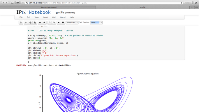
Over at the SIAM blog, Don MacMillen, demonstrates how its now possible, trivial even, to rewrite the entire chapter as an IPython notebook with all MATLAB code replaced with Python.
The notebook is available as a gist and can be viewed statically on nbviewer.
What other examples of successful MATLAB->Python conversions have you found?
The IPython project started as a procrastination task for Fernando Perez during his PhD and is currently one of the most exciting and important pieces of software in computational science today. Last month, Fernando joined us at The University of Manchester after being invited by Nick Higham of the department of Mathematics under the auspices of the EPSRC Network Numerical Algorithms and High Performance Computing
While at Manchester, Fernando gave a couple of talks and we captured one of them using the University of Manchester Lecture Podcasting Service (itself based on a Python project). Check it out below.
This is a guest article written by friend and colleague, Ian Cottam. For part 1, see https://www.walkingrandomly.com/?p=5435
So why do computer scientists use (i != N) rather than the more common (i < N)?
When I said the former identifies “computer scientists” from others, I meant programmers who have been trained in the use of non-operational formal reasoning about their programs. It’s hard to describe that in a sentence or two, but it is the use of formal logic to construct-by-design and argue the correctness of programs or fragments of programs. It is non-operational because the meaning of a program fragment is derived (only) from the logical meaning of the statements of the programming language. Formal predicate logic is extended by extra rules that say what assignments, while loops, etc., mean in terms of logical proof rules for them.
A simple, and far from complete, example is what role the guard in a while/for loop condition in C takes.
for (i= 0; i != N; ++i) {
/* do stuff with a[i] */
}
without further thought (i.e. I just use the formal rule that says on loop termination the negation of the loop guard holds), I can now write:
for (i= 0; i != N; ++i) {
/* do stuff with a[i] */
}
/* Here: i == N */
which may well be key to reasoning that all N elements of the array have been processed (and no more). (As I said, lots of further formal details omitted.)
Consider the common form:
for (i= 0; i < N; ++i) {
/* do stuff with a[i] */
}
without further thought, I can now (only) assert:
for (i= 0; i < N; ++i) {
/* do stuff with a[i] */
}
/* Here: i >= N */
That is, I have to examine the loop to conclude the condition I really need in my reasoning: i==N.
Anyway, enough of logic! Let’s get operational again. Some programmers argue that i<N is more “robust” – in some, to me, strange sense – against errors. This belief is a nonsense and yet is widely held.
Let’s make a slip up in our code (for an example where the constant N is 9) in our initialisation of the loop variable i.
for (i= 10; i != N; ++i) {
/* do stuff with a[i] */
}
Clearly the body of my loop is entered, executed many many times and will quite likely crash the program. (In C we can’t really say what will happen as “undefined behaviour” means exactly that, but you get the picture.)
My program fragment breaks as close as possible to where I made the slip, greatly aiding me in finding it and making the fix required.
Now. . .the popular:
for (i= 10; i<N; ++i) {
/* do stuff with a[i]
}
Here, my slip up in starting i at 10 instead of 0 goes (locally) undetected, as the loop body is never executed. Millions of further statements might be executed before something goes wrong with the program. Worse, it may even not crash later but produce an answer you believe to be correct.
I find it fascinating that if you search the web for articles about this the i<N form is often strongly argued for on the grounds that it avoids a crash or undefined behaviour. Perhaps, like much of probability theory, this is one of those bits of programming theory that is far from intuitive.
Giants of programming theory, such as David Gries and Edsger Dijkstra, wrote all this up long ago. The most readable account (to me) came from Gries, building on Dijkstra’s work. I remember paying a lot of money for his book – The Science of Programming – back in 1981. It is now freely available online. See page 181 for his wording of the explanation above. The Science of Programming is an amazing book. It contains both challenging formal logic and also such pragmatic advice as “in languages that use the equal sign for assignment, use asymmetric layout to make such standout. In C we would write
var= expr;
rather than
var = expr; /* as most people again still do */
The visible signal I get from writing var= expr has stopped me from ever making the = for == mistake in C-like languages.
This is a guest article written by friend and colleague, Ian Cottam.
This brief guest piece for Walking Randomly was inspired by reading about some of the Hackday outputs at the recent SSI collaborative workshop CW14 held in Oxford. I wasn’t there, but I gather that some of the outputs from the day examined source code for various properties (perhaps a little tongue-in-cheek in some cases).
So, my also slightly tongue-in-cheek question is “Given a piece of source code written in a language with “while loops”: how do you know if the author is a computer scientist by education/training?”
I’ll use C as my language and note that “for loops” in C are basically syntactic sugar for while loops (allowing one to gather the initialisation, guard and increment parts neatly together). In other languages “for loops” are closer to Fortran’s original iterative “do loop”. Also, I will work with that subset of code fragments that obey traditional structured (one-entry, one-exit) programming constructs. If I didn’t, perhaps one could argue, as famously Dijkstra originally did, that the density of “goto” statements, even when spelt “break” or “continue”, etc., might be a deciding quality factor.
(Purely as an aside, I note that Linux (and related free/open source) contributors seem to use goto fairly freely as an exception case mechanism; and they might well have a justification. The density of gotos in Apple’s SSL code was illustrated recently by the so-called “goto fail” bug. See also Knuth’s famous article on this subject.)
In my own programming, I know from experience that if I use a goto, I find it so much more difficult to reason logically (and non-operationally) about my code that I avoid them. Whenever I have used a programming language without the goto statement, I have never missed it.
Now, finally to the point at hand, suppose one is processing the elements of an array of single dimension and of length N. The C convention is that the index goes from 0 to N-1. Code fragment A below is written by a non computer scientist, whereas B is.
/* Code fragment A */
for (i= 0; i < N; ++i) {

/* do stuff with a[i] */

}
/* Code fragment B */
for (i= 0; i != N; ++i) {

/* do stuff with a[i] */

}
The only difference is the loop’s guard: i<N versus i!=N.
As a computer scientist by training I would always write B; which would you write?
I would – and will in a follow-up – argue that B is better even though I am not saying that code fragment A is incorrect. Also in the follow-up I will acknowledge the computer scientist who first pointed this out – at least to me – some 33 years ago.
A colleague recently sent me the following code snippet in R
> a=c(1,2,3,40)
> b=a[1:10]
> b
[1]  1  2  3 40 NA NA NA NA NA NA
The fact that R didn’t issue a warning upset him since exceeding array bounds, as we did when we created b, is usually a programming error.
I’m less concerned and simply file the above away in an area of my memory entitled ‘Odd things to remember about R’ — I find that most programming languages have things that look odd when you encounter them for the first time. With that said, I am curious as to why the designers of R thought that the above behaviour was a good idea.
Does anyone have any insights here?
Research Software Engineers (RSEs) are the people who develop software in academia: the ones who write code, but not papers. The Software Sustainability Institute (a group of which I am a Fellow) believes that Research Software Engineers lack the recognition and reward they deserve for their contribution to research. A campaign website – with more information – launched last week:
The campaign has had some early successes and has been generating publicity for the cause, but nothing will change unless the Institute can show that a significant number of Research Software Engineers exist.
Hence this post. If you agree with the issues and objectives on the website, please sign up to the mailing list. If you know of any other Research Software Engineers, please pass this post onto them.
A lot of people don’t seem to know this….and they should. When working with floating point arithmetic, it is not necessarily true that a+(b+c) = (a+b)+c. Here is a demo using MATLAB
>> x=0.1+(0.2+0.3);
>> y=(0.1+0.2)+0.3;
>> % are they equal?
>> x==y

ans =
     0

>> % lets look
>> sprintf('%.17f',x)
ans =
0.59999999999999998

>> sprintf('%.17f',y)
ans =
0.60000000000000009
These results have nothing to do with the fact that I am using MATLAB. Here’s the same thing in Python
>>> x=(0.1+0.2)+0.3
>>> y=0.1+(0.2+0.3)
>>> x==y
False
>>> print('%.17f' %x)
0.60000000000000009
>>> print('%.17f' %y)
0.59999999999999998
If this upsets you, or if you don’t understand why, I suggest you read the following
Does anyone else out there have suggestions for similar resources on this topic?
Consider the following code
function testpow()
%function to compare integer powers with repeated multiplication

rng default
a=rand(1,10000000)*10;

disp('speed of ^4 using pow')
tic;test4p = a.^4;toc
disp('speed of ^4 using multiply')
tic;test4m = a.*a.*a.*a;toc

disp('maximum difference in results');
max_diff = max(abs(test4p-test4m))

end
On running it on my late 2013 Macbook Air with a Haswell Intel i5 using MATLAB 2013b, I get the following results
speed of ^4 using pow
Elapsed time is 0.527485 seconds.
speed of ^4 using multiply
Elapsed time is 0.025474 seconds.
maximum difference in results
max_diff =
   1.8190e-12
In this case (derived from a real-world case), using repeated multiplication is around twenty times faster than using integer powers in MATLAB. This leads to some questions:-
- Why the huge speed difference?
- Would a similar speed difference be seen in other systems–R, Python, Julia etc?
- Would we see the same speed difference on other operating systems/CPUs?
- Are there any numerical reasons why using repeated multiplication instead of integer powers is a bad idea?
I occasionally get emails from researchers saying something like this
‘My MATLAB code takes a week to run and the cleaner/cat/my husband keeps switching off my machine before it’s completed — could you help me make the code go faster please so that I can get my results in between these events’
While I am more than happy to try to optimise the code in question, what these users really need is some sort of checkpointing scheme. Checkpointing is also important for users of high performance computing systems that limit the length of each individual job.
The solution – Checkpointing (or ‘Assume that your job will frequently be killed’)
The basic idea behind checkpointing is to periodically save your program’s state so that, if it is interrupted, it can start again where it left off rather than from the beginning. In order to demonstrate some of the principals involved, I’m going to need some code that’s sufficiently simple that it doesn’t cloud what I want to discuss. Let’s add up some numbers using a for-loop.
%addup.m
%This is not the recommended way to sum integers in MATLAB -- we only use it here to keep things simple
%This version does NOT use checkpointing

mysum=0;
for count=1:100
    mysum = mysum + count;
    pause(1);           %Let's pretend that this is a complicated calculation
    fprintf('Completed iteration %d \n',count);
end

fprintf('The sum is %f \n',mysum);
Using a for-loop to perform an addition like this is something that I’d never usually suggest in MATLAB but I’m using it here because it is so simple that it won’t get in the way of understanding the checkpointing code.
If you run this program in MATLAB, it will take about 100 seconds thanks to that pause statement which is acting as a proxy for some real work. Try interrupting it by pressing CTRL-C and then restart it. As you might expect, it will always start from the beginning:
>> addup
Completed iteration 1
Completed iteration 2
Completed iteration 3
Operation terminated by user during addup (line 6)

>> addup
Completed iteration 1
Completed iteration 2
Completed iteration 3
Operation terminated by user during addup (line 6)
This is no big deal when your calculation only takes 100 seconds but is going to be a major problem when the calculation represented by that pause statement becomes something like an hour rather than a second.
Let’s now look at a version of the above that makes use of checkpointing.
%addup_checkpoint.m
if exist( 'checkpoint.mat','file' ) % If a checkpoint file exists, load it
    fprintf('Checkpoint file found - Loading\n');
    load('checkpoint.mat')

else %otherwise, start from the beginning
    fprintf('No checkpoint file found - starting from beginning\n');
    mysum=0;
    countmin=1;
end

for count = countmin:100
    mysum = mysum + count;
    pause(1);           %Let's pretend that this is a complicated calculation

    %save checkpoint
    countmin = count+1;  %If we load this checkpoint, we want to start on the next iteration
    fprintf('Saving checkpoint\n');
    save('checkpoint.mat');

    fprintf('Completed iteration %d \n',count);
end
fprintf('The sum is %f \n',mysum);
Before you run the above code, the checkpoint file checkpoint.mat does not exist and so the calculation starts from the beginning. After every iteration, a checkpoint file is created which contains every variable in the MATLAB workspace. If the program is restarted, it will find the checkpoint file and continue where it left off. Our code now deals with interruptions a lot more gracefully.
>> addup_checkpoint
No checkpoint file found - starting from beginning
Saving checkpoint
Completed iteration 1
Saving checkpoint
Completed iteration 2
Saving checkpoint
Completed iteration 3
Operation terminated by user during addup_checkpoint (line 16)

>> addup_checkpoint
Checkpoint file found - Loading
Saving checkpoint
Completed iteration 4
Saving checkpoint
Completed iteration 5
Saving checkpoint
Completed iteration 6
Operation terminated by user during addup_checkpoint (line 16)
Note that we’ve had to change the program logic slightly. Our original loop counter was
for count = 1:100
In the check-pointed example, however, we’ve had to introduce the variable countmin
for count = countmin:100
This allows us to start the loop from whatever value of countmin was in our last checkpoint file. Such minor modifications are often necessary when converting code to use checkpointing and you should carefully check that the introduction of checkpointing does not introduce bugs in your code.
Don’t checkpoint too often
The creation of even a small checkpoint file is a time consuming process. Consider our original addup code but without the pause command.
%addup_nopause.m
%This version does NOT use checkpointing
mysum=0;
for count=1:100
    mysum = mysum + count;
    fprintf('Completed iteration %d \n',count);
end
fprintf('The sum is %f \n',mysum);
On my machine, this code takes 0.0046 seconds to execute. Compare this to the checkpointed version, again with the pause statement removed.
%addup_checkpoint_nopause.m

if exist( 'checkpoint.mat','file' ) % If a checkpoint file exists, load it
    fprintf('Checkpoint file found - Loading\n');
    load('checkpoint.mat')

else %otherwise, start from the beginning
    fprintf('No checkpoint file found - starting from beginning\n');
    mysum=0;
    countmin=1;
end

for count = countmin:100
    mysum = mysum + count;

    %save checkpoint
    countmin = count+1;  %If we load this checkpoint, we want to start on the next iteration
    fprintf('Saving checkpoint\n');
    save('checkpoint.mat');

    fprintf('Completed iteration %d \n',count);
end
fprintf('The sum is %f \n',mysum);
This checkpointed version takes 0.85 seconds to execute on the same machine — Over 180 times slower than the original! The problem is that the time it takes to checkpoint is long compared to the calculation time.
If we make a modification so that we only checkpoint every 25 iterations, code execution time comes down to 0.05 seconds:
%Checkpoint every 25 iterations

if exist( 'checkpoint.mat','file' ) % If a checkpoint file exists, load it
    fprintf('Checkpoint file found - Loading\n');
    load('checkpoint.mat')

else %otherwise, start from the beginning
    fprintf('No checkpoint file found - starting from beginning\n');
    mysum=0;
    countmin=1;
end

for count = countmin:100
    mysum = mysum + count;
    countmin = count+1;  %If we load this checkpoint, we want to start on the next iteration

    if mod(count,25)==0
        %save checkpoint
        fprintf('Saving checkpoint\n');
        save('checkpoint.mat');
    end

    fprintf('Completed iteration %d \n',count);
end
fprintf('The sum is %f \n',mysum);
Of course, the issue now is that we might lose more work if our program is interrupted between checkpoints. Additionally, in this particular case, the mod command used to decide whether or not to checkpoint is more expensive than simply performing the calculation but hopefully that isn’t going to be the case when working with real world calculations.
In practice, we have to work out a balance such that we checkpoint often enough so that we don’t stand to lose too much work but not so often that our program runs too slowly.
Checkpointing code that involves random numbers
Extra care needs to be taken when running code that involves random numbers. Consider a modification of our checkpointed adding program that creates a sum of random numbers.
%addup_checkpoint_rand.m
%Adding random numbers the slow way, in order to demo checkpointing
%This version has a bug

if exist( 'checkpoint.mat','file' ) % If a checkpoint file exists, load it
    fprintf('Checkpoint file found - Loading\n');
    load('checkpoint.mat')

else %otherwise, start from the beginning
    fprintf('No checkpoint file found - starting from beginning\n');
    mysum=0;
    countmin=1;
    rng(0);     %Seed the random number generator for reproducible results
end

for count = countmin:100
    mysum = mysum + rand();
    countmin = count+1;  %If we load this checkpoint, we want to start on the next iteration
    pause(1); %pretend this is a complicated calculation

    %save checkpoint
    fprintf('Saving checkpoint\n');
    save('checkpoint.mat');

    fprintf('Completed iteration %d \n',count);
end
fprintf('The sum is %f \n',mysum);
In the above, we set the seed of the random number generator to 0 at the beginning of the calculation. This ensures that we always get the same set of random numbers and allows us to get reproducible results. As such, the sum should always come out to be 52.799447 to the number of decimal places used in the program.
The above code has a subtle bug that you won’t find if your testing is confined to interrupting using CTRL-C and then restarting in an interactive session of MATLAB. Proceed that way, and you’ll get exactly the sum you’ll expect : 52.799447. If, on the other hand, you test your code by doing the following
- Run for a few iterations
- Interrupt with CTRL-C
- Restart MATLAB
- Run the code again, ensuring that it starts from the checkpoint
You’ll get a different result. This is not what we want!
The root cause of this problem is that we are not saving the state of the random number generator in our checkpoint file. Thus, when we restart MATLAB, all information concerning this state is lost. If we don’t restart MATLAB between interruptions, the state of the random number generator is safely tucked away behind the scenes.
Assume, for example, that you stop the calculation running after the third iteration. The random numbers you’d have consumed would be (to 4 d.p.)
0.8147
0.9058
0.1270
Your checkpoint file will contain the variables mysum, count and countmin but will contain nothing about the state of the random number generator. In English, this state is something like ‘The next random number will be the 4th one in the sequence defined by a starting seed of 0.’
When we restart MATLAB, the default seed is 0 so we’ll be using the right sequence (since we explicitly set it to be 0 in our code) but we’ll be starting right from the beginning again. That is, the 4th,5th and 6th iterations of the summation will contain the first 3 numbers in the stream, thus double counting them, and so our checkpointing procedure will alter the results of the calculation.
In order to fix this, we need to additionally save the state of the random number generator when we save a checkpoint and also make correct use of this on restarting. Here’s the code
%addup_checkpoint_rand_correct.m
%Adding random numbers the slow way, in order to demo checkpointing

if exist( 'checkpoint.mat','file' ) % If a checkpoint file exists, load it
    fprintf('Checkpoint file found - Loading\n');
    load('checkpoint.mat')

    %use the saved RNG state
    stream = RandStream.getGlobalStream;
    stream.State = savedState;

else % otherwise, start from the beginning
    fprintf('No checkpoint file found - starting from beginning\n');
    mysum=0;
    countmin=1;
    rng(0);     %Seed the random number generator for reproducible results
end

for count = countmin:100
    mysum = mysum + rand();
    countmin = count+1;  %If we load this checkpoint, we want to start on the next iteration
    pause(1); %pretend this is a complicated calculation

    %save the state of the random number genertor
    stream = RandStream.getGlobalStream;
    savedState = stream.State;
    %save checkpoint
    fprintf('Saving checkpoint\n');
    save('checkpoint.mat');

    fprintf('Completed iteration %d \n',count);
end
fprintf('The sum is %f \n',mysum);
Ensuring that the checkpoint save completes
Events that terminate our code can occur extremely quickly — a powercut for example. There is a risk that the machine was switched off while our check-point file was being written. How can we ensure that the file is complete?
The solution, which I found on the MATLAB checkpointing page of the Liverpool University Condor Pool site is to first write a temporary file and then rename it. That is, instead of
save('checkpoint.mat')/pre>
we do
if strcmp(computer,'PCWIN64') || strcmp(computer,'PCWIN')
            %We are running on a windows machine
            system( 'move /y checkpoint_tmp.mat checkpoint.mat' );
else
            %We are running on Linux or Mac
            system( 'mv checkpoint_tmp.mat checkpoint.mat' );
end
As the author of that page explains ‘The operating system should guarantee that the move command is “atomic” (in the sense that it is indivisible i.e. it succeeds completely or not at all) so that there is no danger of receiving a corrupt “half-written” checkpoint file from the job.’
Only checkpoint what is necessary
So far, we’ve been saving the entire MATLAB workspace in our checkpoint files and this hasn’t been a problem since our workspace hasn’t contained much. In general, however, the workspace might contain all manner of intermediate variables that we simply don’t need in order to restart where we left off. Saving the stuff that we might not need can be expensive.
For the sake of illustration, let’s skip 100 million random numbers before adding one to our sum. For reasons only known to ourselves, we store these numbers in an intermediate variable which we never do anything with. This array isn’t particularly large at 763 Megabytes but its existence slows down our checkpointing somewhat. The correct result of this variation of the calculation is 41.251376 if we set the starting seed to 0; something we can use to test our new checkpoint strategy.
Here’s the code
% A demo of how slow checkpointing can be if you include large intermediate variables

if exist( 'checkpoint.mat','file' ) % If a checkpoint file exists, load it
    fprintf('Checkpoint file found - Loading\n');
    load('checkpoint.mat')
    %use the saved RNG state
    stream = RandStream.getGlobalStream;
    stream.State = savedState;
else %otherwise, start from the beginning
    fprintf('No checkpoint file found - starting from beginning\n');
    mysum=0;
    countmin=1;
    rng(0);     %Seed the random number generator for reproducible results
end

for count = countmin:100
    %Create and store 100 million random numbers for no particular reason
    randoms = rand(10000);
    mysum = mysum + rand();
    countmin = count+1;  %If we load this checkpoint, we want to start on the next iteration
    fprintf('Completed iteration %d \n',count);

    if mod(count,25)==0
        %save the state of the random number generator
        stream = RandStream.getGlobalStream;
        savedState = stream.State;
        %save and time checkpoint
        tic
        save('checkpoint_tmp.mat');
        if strcmp(computer,'PCWIN64') || strcmp(computer,'PCWIN')
            %We are running on a windows machine
            system( 'move /y checkpoint_tmp.mat checkpoint.mat' );
        else
            %We are running on Linux or Mac
            system( 'mv checkpoint_tmp.mat checkpoint.mat' );
        end
        timing = toc;
        fprintf('Checkpoint save took %f seconds\n',timing);
    end

end
fprintf('The sum is %f \n',mysum);
On my Windows 7 Desktop, each checkpoint save takes around 17 seconds:
Completed iteration 25
        1 file(s) moved.
Checkpoint save took 17.269897 seconds
It is not necessary to include that huge random matrix in a checkpoint file. If we are explicit in what we require, we can reduce the time taken to checkpoint significantly. Here, we change
save('checkpoint_tmp.mat');
to
save('checkpoint_tmp.mat','mysum','countmin','savedState');
This has a dramatic effect on check-pointing time:
Completed iteration 25
        1 file(s) moved.
Checkpoint save took 0.033576 seconds
Here’s the final piece of code that uses everything discussed in this article
%Final checkpointing demo

if exist( 'checkpoint.mat','file' ) % If a checkpoint file exists, load it
    fprintf('Checkpoint file found - Loading\n');
    load('checkpoint.mat')
    %use the saved RNG state
    stream = RandStream.getGlobalStream;
    stream.State = savedState;
else %otherwise, start from the beginning
    fprintf('No checkpoint file found - starting from beginning\n');
    mysum=0;
    countmin=1;
    rng(0);     %Seed the random number generator for reproducible results
end

for count = countmin:100
    %Create and store 100 million random numbers for no particular reason
    randoms = rand(10000);
    mysum = mysum + rand();
    countmin = count+1;  %If we load this checkpoint, we want to start on the next iteration
    fprintf('Completed iteration %d \n',count);

    if mod(count,25)==0 %checkpoint every 25th iteration
        %save the state of the random number generator
        stream = RandStream.getGlobalStream;
        savedState = stream.State;
        %save and time checkpoint
        tic
        %only save the variables that are strictly necessary
        save('checkpoint_tmp.mat','mysum','countmin','savedState');
        %Ensure that the save completed
        if strcmp(computer,'PCWIN64') || strcmp(computer,'PCWIN')
            %We are running on a windows machine
            system( 'move /y checkpoint_tmp.mat checkpoint.mat' );
        else
            %We are running on Linux or Mac
            system( 'mv checkpoint_tmp.mat checkpoint.mat' );
        end
        timing = toc;
        fprintf('Checkpoint save took %f seconds\n',timing);
    end

end
fprintf('The sum is %f \n',mysum);
Parallel checkpointing
If your code includes parallel regions using constructs such as parfor or spmd, you might have to do more work to checkpoint correctly. I haven’t considered any of the potential issues that may arise in such code in this article
Checkpointing checklist
Here’s a reminder of everything you need to consider
- Test to ensure that the introduction of checkpointing doesn’t alter results
- Don’t checkpoint too often
- Take care when checkpointing code that involves random numbers – you need to explicitly save the state of the random number generator.
- Take measures to ensure that the checkpoint save is completed
- Only checkpoint what is necessary
- Code that includes parallel regions might require extra care
A question I get asked a lot is ‘How can I do nonlinear least squares curve fitting in X?’ where X might be MATLAB, Mathematica or a whole host of alternatives. Since this is such a common query, I thought I’d write up how to do it for a very simple problem in several systems that I’m interested in
This is the Julia version. For other versions,see the list below
- Simple nonlinear least squares curve fitting in Maple
- Simple nonlinear least squares curve fitting in Mathematica
- Simple nonlinear least squares curve fitting in MATLAB
- Simple nonlinear least squares curve fitting in Python
- Simple nonlinear least squares curve fitting in R
The problem
xdata = -2,-1.64,-1.33,-0.7,0,0.45,1.2,1.64,2.32,2.9
ydata = 0.699369,0.700462,0.695354,1.03905,1.97389,2.41143,1.91091,0.919576,-0.730975,-1.42001
and you’d like to fit the function

using nonlinear least squares. You’re starting guesses for the parameters are p1=1 and P2=0.2
For now, we are primarily interested in the following results:
- The fit parameters
- Sum of squared residuals
Future updates of these posts will show how to get other results such as confidence intervals. Let me know what you are most interested in.
Julia solution using Optim.jl
Optim.jl is a free Julia package that contains a suite of optimisation routines written in pure Julia. If you haven’t done so already, you’ll need to install the Optim package
Pkg.add("Optim")
The solution is almost identical to the example given in the curve fitting demo of the Optim.jl readme file:
using Optim

model(xdata,p) = p[1]*cos(p[2]*xdata)+p[2]*sin(p[1]*xdata)

xdata = [-2,-1.64,-1.33,-0.7,0,0.45,1.2,1.64,2.32,2.9]
ydata = [0.699369,0.700462,0.695354,1.03905,1.97389,2.41143,1.91091,0.919576,-0.730975,-1.42001]

beta, r, J = curve_fit(model, xdata, ydata, [1.0, 0.2])
# beta = best fit parameters
# r = vector of residuals
# J = estimated Jacobian at solution

@printf("Best fit parameters are: %f and %f",beta[1],beta[2])
@printf("The sum of squares of residuals is %f",sum(r.^2.0))
The result is
Best fit parameters are: 1.881851 and 0.700230
@printf("The sum of squares of residuals is %f",sum(r.^2.0))
Notes
I used Julia version 0.2 on 64bit Windows 7 to run the code in this post