
Archive for the ‘programming’ Category
I read a lot of blogs concerning topics such as numerical computing, programming and computer algebra and most of the time the subject matter can be a bit…well…hard! The articles concerned can often be interesting and very useful but it can take a heck of a lot of concentration on my part before I can properly grok what the author is trying to say.
Sometimes though I come across something that is both useful and interesting and also so mind-numblingly simple that I wonder why on earth I didn’t think of it before. A case in point is Loren’s recent “Art of Matlab” article called “Should min and max marry?”.
I won’t re-iterate what she has written since she has done a great job and makes her point well. I am also currently busy implementing her idea in a piece of code I am writing at the moment while pretending to everyone around me that its such an obvious idea that I had thought about it well in advance!
At some point in the future I am going to need to do some Java programing for work-related purposes and so I thought I should set up my Ubuntu based laptop for Java development. Everything you need to do this are in the Ubuntu repositories so the installation went without incident but I hit a brick wall when I tried to compile and run this very simple program
class myfirstjavaprog
{
   public static void main(String args[])
   {
      System.out.println("Hello World");
   }
}
I compiled this with the command
javac myfirstjavaprog.java
The .class file was produced without any problems but when I tried to run it with
java myfirstjavaprog
I got a hideous looking error message that started off like this
exception in thread “main” java.lang.UnsupportedClassVersionError: Bad version number in .class file
at java.lang.ClassLoader.defineClass1(Native Method)
at java.lang.ClassLoader.defineClass(ClassLoader.java:620)
at java.security.SecureClassLoader.defineClass(SecureClassLoader.java:124)
All that for a Hello World program! This was not a good start but it turns out that there is an easy fix. The version of Java being used by my java command was different from that being used by my javac command and they need to be the same. The commands that allow you to configure Java versions on Ubuntu are
sudo update-alternatives –config java
sudo update-alternatives –config javac
Ensure that they are set to use the same version and you should be good to go.
In a recent post over at 360 the author was discussing how Joe Turner (a prof of musical composition) has formed a musical composition based on the expansion of Pi in base 12 and it sounds pretty good considering the fact that it is based on a random sequence. This was picked up by another blog I discovered recently (thanks to the carnival of mathematics) where the author asked if anyone else would mind producing similar compositions based on other mathematical constants.
On the train journey home from work I thought that I might be able to get Mathematica to produce simplified versions of these sort of compositions without too much effort. So I fired up my copy of Mathematica, plugged in some headphones (I was fairly sure that my fellow commuters would not appreciate the music of Pi as much as I) and set to work. Although I knew that Mathematica had sound capabilities I had never used them before so the help browser (as usual) was indispensable.
I am going to present the rest of this post as a tutorial, with Mathematica commands in bold followed by the output in normal tyle. This is my first attempt at a tutorial in a blog post so feedback would be welcomed.
From the help browser I discovered that you can represent a note in Mathematica using SoundNote. Middle C is represented by SoundNote[0], one semi-tone above middle C is SoundNote[1] , a whole tone above Middle C is SoundNote[2] and so on. You can also use negative numbers so that SoundNote[-1] is one semi-tone below middle C for example.
So far so good but I don’t want to just represent the notes symbolically – I want to actually play them. The way to do this is by wrapping a SoundNote expression with Sound[]. So to play a middle C just evaluate
Sound[SoundNote[0]]
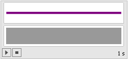
A little interface appears that looks like the graphic above and when you click the play button (represented by a triangle) you will hear a piano sample at middle C that lasts for one second.
So far so good – I have a way of playing any integer I choose but I need to be able to play a list of notes if I am going to convert Pi to music. For those of you who don’t know much about Mathematica all you need to do to create a list of ANYTHING is separate them by commas and wrap the whole thing in curly braces {} so a list the integers 1 to 5 looks like this
{1,2,3,4,5}
A list of strings looks like this
{“hello”,”world”,”these”,”are”,”strings”}
Finally, a list of three SoundNotes looks like this:
{SoundNote[3], SoundNote[1], SoundNote[4]}
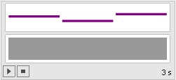
Wrap this list with Sound[] to play the three notes in sequence:
Sound[{SoundNote[3], SoundNote[1], SoundNote[4]}]
So all I need now is to get the digits of Pi (or any other number I might choose) into a list of SoundNotes. If all I wanted was the decimal expansion of Pi to any number of digits I choose then I could use the N command:
N[Pi,20]
3.1415926535897932385
Since the original article asks for Pi in base twelve I could use BaseForm[number,base] to display Pi in base 12 as follows:
BaseForm[N[Pi,20],12]
3.184809493b9186645712
This is all well and good but what I actually want is a list of the digits of Pi in base 12 and so I am going to use the RealDigits command which has the syntax RealDigits[number,base,number_of_digits]. This returns a list of the digits of your number according to your specified base and number of digits. So to get a list of the first 20 digits of Pi in base 12 I do
RealDigits[Pi, 12, 20]
{{3, 1, 8, 4, 8, 0, 9, 4, 9, 3, 11, 9, 1, 8, 6, 6, 4, 5, 7, 3}, 1}
Now this result is not just a simple list but is list of lists instead. The first element is a list of the digits of Pi in base 12 and the second element is the number of digits to the left of the decimal point. I only want the first element of this list of lists – namely the list of digits of Pi. To extract elements from lists in Mathematica you use double square brackets [[ ]] so to get the 3rd element of the list {1,4,9,16,25} you would type
{1,4,9,16,25}[[3]]
9
So to get that first list from the result of RealDigits[Pi, 12, 20] we do
RealDigits[Pi, 12, 20][[1]]
{3, 1, 8, 4, 8, 0, 9, 4, 9, 3, 11, 9, 1, 8, 6, 6, 4, 5, 7, 3}
So far so good but we are not done yet – somehow I need to wrap each integer in this list with SoundNote[]. One way to do this is by using Map[]. For example I can wrap each element of the list {3,1,4} with SoundNote by doing
Map[SoundNote,{3,1,4}]
{SoundNote[3], SoundNote[1], SoundNote[4]}
Applying this knowledge to the code we have built up so far allows us to write the following
Map[SoundNote,

RealDigits[Pi, 12, 20][[1]]

]
{SoundNote[3], SoundNote[1], SoundNote[8], SoundNote[4], SoundNote[8],SoundNote[0], SoundNote[9], SoundNote[4], SoundNote[9],SoundNote[3], SoundNote[11], SoundNote[9], SoundNote[1],SoundNote[8], SoundNote[6], SoundNote[6], SoundNote[4], SoundNote[5],SoundNote[7], SoundNote[3]}
I have started to format my Mathematica commands a bit to make them more readable by using multiple lines. This is not necessary but I find that if I don’t do this then I soon start to loose track of all those square brackets and get into a horrible mess. All that I have to do now is wrap this result with Sound[] and my job is done.
Sound[

Map[SoundNote,

RealDigits[Pi, 12, 20][[1]]

]]

By modifying this group of commands you can ‘play’ any expression you like to as many decimal places as you like but there is still work to be done. For example we are stuck with only using a piano and every note has a one second duration which is far from ideal but this post is getting a bit long so I will explain how to change these in a future post if anyone is interested.
By the time my train journey was over I had produced a little ‘applet’ in Mathematica using the principles described here along with the Manipulate function. It could play Pi in any number base using any one of a range of instruments with variable note speed. I fully intended on refining it a bit and submitting it to the Wolfram Demonstrations project but when I got home and regained internet access I discovered that I had been beaten to it by someone called Hector Zenil. Hector has written a very nice demonstration called Math Songs which does exactly what I had been trying to achieve and a whole lot more. Not only can you listen to Pi but you can also listen to e, Euler’s Gamma constant, the golden ratio, the Catalan constant and a few more I haven’t even heard of.
Oh well…you can’t win them all and Hector has done a fantastic job (better than I would have done to be honest). The best thing is that you don’t even need Mathematica to play with his creation. The free (but rather large) MathPlayer will do the job nicely for you.
So, have fun with Hector’s little demonstration and I hope the mini-tutorial here was useful to someone. As always feel free to leave comments.
I have a couple of perl projects that make use of the GD::Graph module and I needed to set them up on a new machine. I was expecting to install the module without any problems but I was wrong. With a live internet connection I started off by starting the CPAN shell by typing the following in a bash shell
sudo perl -MCPAN -e shell
Since it was the first time I had run this command on this particular machine I had to answer a lot of questions but simply selected the defaults for everything as this usually works for me. Once in the CPAN shell I entered
install Bundle::CPAN
and selected all of the defaults again. Once the CPAN bundle had finished installing I tried to install GD::Graph by typing
install GD::Graph
but it failed with hundreds of errors – the first of which was
GD.xs:7:16: error: gd.h: No such file or directory
This was fixed with the following apt-get command (in the bash shell)
sudo apt-get install libgd2-xpm-dev
back in the CPAN shell I still couldn’t get GD::Graph to build and I guessed this was because of some left over files from the failed build. I don’t know the command to clean things up inside the CPAN shell and am too lazy to read the docs so I simply went into the .cpan/build directory in my home directory and deleted anything that started with GD – eg
rm -rf GD-2.35-HC_vkB
rm -rf GDGraph-1.44-Evfibe
and so on. Those strings at the end (VkB and so on) look random so they might be different on your machine. Then I went back into the CPAN shell and ran
install GD::Graph
again. There were a few dependencies which the script fetched and installed for me but everything worked smoothly. With a bit of luck these notes will be of use to someone else out there – please let me know if this is the case.
Over the years I have programmed in a reasonable number of languages but the ones I am actually using right now are Fortran, C++, Mathematica, Matlab and Perl. The one I would choose would depend on what I needed to accomplish, maybe Fotran for high speed numerics, Matlab for quick numerical algorithm development or Perl for sysadmin work and for the most part this tool-set serves my purposes well.
Just recently, however, I have been getting itchy feet and have been wanting to learn another programming language as it is a process I quite enjoy and last time I did it (with Perl) it turned out to be pretty useful. The question, of course, is which one to choose? I want a language that is going to be fun to use (to keep up my interest) and useful in my day job (so I can justify the time spent).
For me, one language stuck out more than all of the others – Python. I have always been dimly aware of it but until recently you could summarize my knowledge of it as follows
- It’s free
- It’s not a traditional compiled language (like C or Fortran) – it uses bytecodes and a virtual machine like Java
- It’s the one where white space matters
- Perl and Python people argue a lot
More recently, however, I have discovered a few more things about it piqued my interest.
- The open source CAS system – SAGE – is implemented in Python
- There are mature python libraries for doing numerical computing – numpy and scipy
- There is a wonderful looking matlab-like plotting library for it – matplotlib
- There are a lot of scientific applications developed using it
- I can install it on my mobile phone
- There is a number-theoretic (another emerging interest I have) library for it – NZMATH
So python it is then. Although there are a lot of great looking python tutorials on the web, I prefer to do my learning from a book, I am showing my age I guess. When I was learning Perl I used the O’Reilly book, learning perl, and would recommend it to any new Perl learners without hesitation. Since they have served me so well in the past, I turned to O’Reilley again and have just bought Learning Python (below) from Amazon. If you would like to join me on my Python journey (and support this site) then click on the image below and buy a copy.

According to the server logs one of the most popular posts I have made on Walking Randomly is the one I made a couple of months ago about the Logo programming language. Of course this may be due to the fact that this year marked the 40th anniversary of the language thus leading people to google for nostalgic reasons but it may also be because it is a genuinely interesting language. One thing that’s for certain is that programming in Logo can be a lot of fun and naturally leads to further study of concepts such as recursion, geometry and fractals.
With this in mind I thought it was high time I worked out a way of installing Logo on the pocket PC so that I can play with it on my new toy – the remarkable HTC TyTyn II My task set, I embarked on a set of very extensive google searches and to my surprise came up with very little.
The only native windows mobile solution that I could find was a free package called pocket turtle by Morten of Xpoint.dk. Although very much in the alpha stages of development (It only supports 6 commands and no user defined functions) this software looked promising and so I contacted the author to ask what he plans to do with it. His reply was prompt and friendly but unfortunately his future plans do not include any more pocket turtle development which is a shame but understandable since developing free software is a very time consuming affair. I tried to install it anyway since a little Logo is better than none at all but unfortunately could not get it on my new Windows Mobile 6 device.
Things were looking bleak on the pocket-pc logo front. Just as I was about to give up and resign myself to using my laptop to quench my Logo thirst, I came across a package called TinyLogo which was developed quite a while ago now. It is free, which is nice, but unfortunatley it only runs on PalmOS hardware. Now this is great news for the Palm users out there (Amanda – are you taking note of this?) but not so good for the likes of me.
A fantastic piece of (nonfree) software called StyleTap came to my rescue. Essentially what this does is emulate the Palm OS operating system on Windows Mobile devices so now you can run all of those must have Palm programs (such as TinyLogo) on your pocket PC.
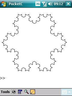
I installed the trial version of StyleTap then installed TinyLogo on top of that and it worked like a charm. The TinyLogo icon appears on my device exactly as if it were a native application and the only way I can tell that this is not the case is that the menus look a little old fashioned (just like Palm OS) when I use it.
A quick read of the TinyLogo documentation later (recommended since the interface is not very intuitive in my opinion) and I was cooking on gas as the following screenshots demonstrate.

There is one minor problem. In order to write and edit TinyLogo scripts you need to use the standard PalmOS application ‘MemoPad’ and this is not included with StyleTap – probably for copyright reasons. All is not lost, however, since it turns out that MemoPad is not very good and so many people have developed free MemoPad replacements. One such example is jpad which also works on StyleTap without a hitch and has the added bonus of looking delightfully old fashioned which somehow enhanced the Logo experience for me.
I was so pleased with the StyleTap emulator that I ended up buying it – not just for TinyLogo you understand (honest) – but because there are quite a few Palm OS applications out there that I would quite like to play with again.
In summary using TinyLogo via StyleTap is a workable (albeit fiddly) solution for Logo enthusiasts who would like to code directly on their pocket PC. The interface is old fashioned and non-intuitive (well it was coded back in 1999 so this is to be expected) and because of this, and the fact that you have to pay for the StyleTap emulator, I would not recommend it for classroom use. Hopefully someone, somewhere will come up with a native Windows Mobile solution but for now TinyLogo on StyleTap is the best we have.
I don’t know very much about PHP. In fact it is probably more accurate to say that I don’t know anything about programming in PHP and yet, earlier today, I found myself in need of being able to type in simple PHP scripts and run them on the command line. A quick google search later and I find that I need to issue the following command in Ubuntu
apt-get install php5-cli
Now I can write little scripts like this one (which I called md5.php) and run them on the command line
#!/usr/bin/php -q
<?php
$arg=$_SERVER["argv"][1];
echo md5($arg),"\n";
?>
./md5.php hello
5d41402abc4b2a76b9719d911017c592
I mention it because I might forget about it and looking up on here is quicker for me than googling it.
One of the great things about browsing the Internet is that you never know where you are going to end up. Recently, I have taken to looking at new entries on the Wolfram Demonstrations page (mentioned in an earlier blog post) and, if I find something interesting, I follow it up. By doing this I have discovered all sorts of delightful (but, it has to be said, mostly useless) mathematical tidbits.
My most recent find is a demonstration entitled ‘Polygons arranged in a circle‘ which produces some attractive looking flower-like designs by drawing a set of identical regular polygons arranged in a circle. The instant I set eyes on the preview I had a sense of deja-vu. Not only had I seen such patterns before but I had written the code to produce them when I was a child of around 10 on a BBC Micro using the Logo programming language. These were probably among the first codes I had ever written in my life and started a lifelong fascination with programming that is still with me today.
The Logo programming language is a dialect of Lisp that was developed in the late 60s by Daniel Bobrow and Wallace Feurzeig of BBN in collaboration with Seymour Papert of MIT. You may not have heard of BBN but, along with developing Logo, they were the company that developed the Arpanet – widely held to be the precursor of the internet. They also put the @ symbol in email addresses by the way.
Back in the 60s it was much harder to program computers than it is now and Logo was developed as a learning tool for children. It was designed not just to help teach programming but also to help teach concepts from mathematics such as geometry and algebra. For more about the history of Logo you might like to read Wallace Feurzeig’s ‘The LOGO Lineage’ -originally published in 1984 as part of the book ‘Digital Deli’.
Although it is a very powerful language (and to get an idea of just how powerful take a look at Brian Harvey’s set of 3 Logo-centric computer science books available for download from here), Logo is best known for it’s Turtle Graphics. The turtle was originally a robot that moved around the floor, holding a pen and controlled by a computer using Logo. These days it is represented by a sprite on a computer screen. Using Logo and the turtle you can write programs to draw anything you like. The commands are simple – for example:
forward 20 – moves forward 20 units
right 90 – rotates to the right 90 degrees
repeat n [ ] – repeat the commands in the brackets n times.
So to draw a square
repeat 4 [forward 20 right 90]
we can also write subroutines – here is one that will draw a hexagon
to hexagon
repeat 6 [forward 20 right 60]
end
We are now just one step from reproducing the type of graphics in the Mathematica demonstration
to flower
repeat 30 [ hexagon right 12]
end
running the command ‘flower’ will produce the pattern below.

With a little thought (and one or 2 extra commands not mentioned here) you can modify the code to produce any of the designs in the Wolfram Demonstration. This is all well and good but how do you get Logo on your PC? I found a great implementation called Berkeley logo – there are many others but this one seems to be among the best. If you have Ubuntu Linux then the command to install it is
sudo apt get install ucblogo
A gentle introduction to the Logo language can be found at the Logo foundation. You should bear in mind that, unlike languages such as C, there is no standard syntax for Logo and so the language varies from implementation to implementation. To get an idea of the number of implementations out there take a look at The Great Logo atlas.
This little investigation started out as a nostalgia trip for me but has ended up being a bit more than that. I thought Logo was a dead language from my past but it seems that it is still very much alive and well. It even has an active usenet group. When I was learning Logo at school we didn’t take it much further than the geometric pictures shown above which is a shame because it is clearly a very powerful language.
Since I already have to keep so many languages in my head for professional reasons, I doubt that I will use Logo for anything serious but will almost certainly be playing with it from time to time. Logo is fun and sometimes I forget that I got into programming in the first place because it can be fun.
I am in the middle of a small project written using the Perl scripting language and I found myself wanting to be able to plot a graph. Now I have faced this problem before and last time I cheated and got my Perl script to talk to the superb open source plotting program, gnuplot. This worked just fine but for various reason I wanted to code the whole thing in Perl itself this time – no talking to external programs.
A bit of googling around and I hit upon the GD::Graph Perl module. Once I had this installed I was producing graphs in .png format in no time. Now the resulting plots are not the prettiest I have ever seen but they do the job and maybe with a bit of tweaking they can be made to look a bit nicer. An example Bar chart is shown below (the text is distorted due to resizing the image – not because that’s how it actually looks)

A lot of sample scripts are included with the package and over at gdgraph.com you can see what all of the resulting plots look like. All in all it’s a nice little package and is still under active development.