
Archive for the ‘programming’ Category
Someone emailed me recently complaining that the ParallelTable function in Mathematica didn’t work. In fact it made his code slower! Let’s take a look at an instance where this can happen and what we can do about it. I’ll make the problem as simple as possible to allow us to better see what is going on.
Let’s say that all we want to do is generate a list of the prime numbers as quickly as possible using Mathematica. The code to generate the first 20 million primes is very straightforward.
primelist = Table[Prime[k], {k, 1, 20000000}];
To time how long this list takes to calculate we can use the AbsoluteTime function as follows.
t = AbsoluteTime[];
primelist = Table[Prime[k], {k, 1, 20000000}];
time2 = AbsoluteTime[] - t
This took about 63 seconds on my machine. Taking a quick look at the Mathematica documentation we can see that the parallel version of Table is, obviously enough, ParallelTable. What could be simpler? So, to spread this calculation over both processors in a dual-core laptop we simply need to do the following
t = AbsoluteTime[];
primelist = ParallelTable[Prime[k], {k, 1, 20000000}];
time2 = AbsoluteTime[] - t
The result? 98 seconds! So, it seems that the parallel version is more than 50% SLOWER! My correspondent was right – ParallelTable doesn’t seem to work at all.
Before we send a message to Wolfram Tech Support though, let’s dig a little deeper. It turns out that a single evaluation of
Prime[k] for any given k is very quick – even for high k. Prime[100000000] evaluates in a tiny fraction of a second for example (try it! – it really is astonishingly quick.)
What I suspect is happening here is that when you move to the parallel version, the kernels spend most of the time communicating with each other rather than actually calculating anything. I think that ParallelTable does something roughly like the following.
Kernel1:Give me a k.
Master:have k=1.
Kernel2:Give me a k.
Master:have k=2
Kernel1:I’ve done k=1 and the answer is 2, give me another k
Master: have k=3
kernel2:I’ve done k=2 and the answer is 3, give me another k etc
So, the kernels spend more time talking about the work that needs to be done rather than actually doing it. Also, for various reasons, kernel1 and kernel2 might get out of sync and so the Master kernel may end up with a list out of order. If so then it will need to reorder the lists at the end of the calculations and so that’s even more time taken.
So, my approach was to try and reduce the amount of communication between kernels to something like
Master: Kernel 1 – you go away and get me first 10 million primes. Don’t bother me until it’s done.
Master: kernel 2 – you go away and get me the second 10 million. Don’t bother me until it’s done.
The following Mathematica code does this.
t = AbsoluteTime[];
job1 = ParallelSubmit[Table[Prime[k], {k, 1, 10000000}]];
job2 = ParallelSubmit[Table[Prime[k], {k, 10000001, 20000000}]];
{a1, a2} = WaitAll[{job1, job2}];
time2 = AbsoluteTime[] - t
This works in 40 seconds compared to the original time of 62 seconds. Not a 2x speedup but not too shabby for so little extra work on our part.
The moral of the story? Make sure that your code spends more time actually doing work than it does just talking about it.
Disclaimer: I am still learning about Mathematica’s parallel tools myself so don’t take this stuff as gospel. Also, there are almost certainly more efficient ways of getting a list of primes than using the Prime[k] function. I am only using Prime[k] here because it is an example of a function that evaluates very quickly.
Back in 1997 I was a 2nd year undergraduate of Physics and I was taught how to program in Fortran, a language that has survived over 40 years due to several facts including
- It is very good at what it does. Well written Fortran code, pushed through the right compiler is screamingly fast.
- There are millions of lines of legacy code still being used in the wild. If you end up doing research in subjects such as Chemistry, Physics or Engineering then you will almost certainly bump into Fortran code (I did!).
- A beginner’s course in Fortran has been part of the staple diet in degrees in Physics, Chemistry and various engineering disciplines (among others) for decades.
- It constantly re-invents itself to include new features. I was taught Fortran 77 (despite it being 1997) but you can now also have your pick of Fortran 90, 95, 2003, and soon 2008.
Almost everyone I knew hated that 1997 Fortran course and the reasons for the hatred essentially boiled down to one of two points depending on your past experience.
- Fortran was too hard! So much work for such small gains (First time – programmers)
- The course was far too easy. It was just a matter of learning Fortran syntax and blitzing through the exercises. (People with prior experience)
The course was followed by a numerical methods course which culminated in a set of projects that had to be solved in Fortran. People hated the follow on course for one of two reasons
- They didn’t have a clue what was going on in the first course and now they were completely lost.
- The problems given were very dull and could be solved too easily. In Excel! Fortran was then used to pass the course.
Do you see a pattern here?
Fast forward to 2009 and I see that Fortran is still being taught to many undergraduates all over the world as their first ever introduction to programming. Bear in mind that these students are used to being able to get interactive 3D plots from the likes of Mathematica, Maple or MATLAB and can solve complex differential equations simply by typing them into Wolfram Alpha on the web. They can solve problems infinitely more complicated then the ones I was faced with in even my most advanced Fortran courses with just a couple of lines of code.
Learn Fortran – spend a semester achieving not very much
These students study subjects such as physics and chemistry because they are interested in the subject matter and computers are just a way of crunching through numbers (and the algebra for that matter) as far as they are concerned. Despite having access to untold amounts of computational and visualisation power coupled with easy programming languages thanks to languages such as MATLAB and Python, these enthusiastic, young potential programmers get forced to bend their minds around the foibles of Fortran.
For many it’s their first ever introduction to programming and they get forced to work with one of the most painful programming languages in existence (in my opinion at least). Looking at a typical one-semester course it seems that by the time they have finished they will be able to produce command line only programs that do things like multiply matrices together (slowly), solve the quadratic equation and find the mean and standard deviation of a list of numbers.
Not particularity impressive for an introduction to the power of computation in their subject is it?
Fortran syntax is rather unforgiving compared to something like Python and it takes many lines of code to achieve even relatively simple results. Don’t believe me? OK, write a program in pure Fortran that gives a plot of a Sin(n*x) for integer n and x ranging from -2*pi to 2*pi. Now connect that plot up to a slider control which will control the value of n. Done? Ok – now get it working on another operating system (eg if you originally used Windows, get it to work on Mac OS X).
Now try the same exercise in Python or Mathematica.
This is still a very basic program but it would give a much greater sense of achievement compared to finding the mean of list of numbers and could easily be extended for more able students (Fourier Series perhaps). I believe that many introductory Fortran programming courses end up teaching students that programming means ‘Calculating things the hard way’ when they should be leaving an introductory course with the opposite impression.
Learn Fortran – and never use it again.
Did you learn Fortran at University? Are you still using it? If you answer yes to both of those questions then there is a high probability that you are still involved in research or that advanced numerical analysis is the mainstay of your job. I know a lot of people in the (non-academic) IT industry – many of them were undergraduates in Physics or Chemistry and so they learned Fortran. They don’t use it anymore. In fact they never used it since completing their 1st semester, 2nd year exam and that includes the computational projects they chose to do as part of their degrees.
The fact of the matter is that most undergraduates in subjects such as Physics end up in careers that have nothing to do with their degree subject and so most of them will never use Fortran ever again. The ‘programming concepts’ they learned might be useful if they end up learning Java, Python or something along those lines but that’s about it. Would it not be more sensible to teach a language that can support the computational concepts required in the underlying subject that also has an outside chance of being used outside of academia?
Teach Fortran – and spend a fortune on compilers
There are free Fortran compilers available but in my experience these are not the ones that get used the most for teaching or research and this is because the commercial Fortran compilers tend to be (or at least,they are perceived to be) much better. The problem is that when you are involved with looking after the software portfolio of a large University (and I am) then no one will agree on what ‘the best’ compiler is. (Very) roughly paraphrased, here are some comments I have received from Fortran programmers and teachers over the last four years or so.
- When you teach Fortran, you MUST use the NAG Fortran compiler since it is the most standards compliant. The site license allows students to have it on their own machines which is useful.
- When you teach Fortran, you MUST use the Silverfrost compiler because it supports Windows GUI programming via Clearwin.
- We MUST avoid the Silverfrost compiler for teaching because it is not available on platforms such as Mac and Linux.
- We MUST avoid the NAG compiler for teaching because although it has a great user interface for Windows, it is command line only for Linux and Mac. This confuses students.
- If we are going to teach Fortran then we simply MUST use the Intel Fortran Compiler. It’s the best and the fastest.
- We need the Intel Fortran Compiler for research because it is the only one compatible with Abaqus.
- A site license for Absoft Fortran is essential. It’s the only one that will compile <insert application here> which is essential for my group’s work.
- We should only ever use free Fortran compilers – relying on commercial offerings is wrong.
I’m only getting started! Choose a compiler, any compiler – I’ll get back to you within the week with an advocate who thinks we should get a site license for it and another who hates it with a passion. Let’s say you had a blank cheque book and you gave everyone exactly what they wanted – your institution would be spending tens of thousands of pounds on Fortran compilers and you’d still be annoying the free-software advocate.
Needless to say, most people don’t have a blank cheque book. At Manchester University (my workplace) we support 2 site-wide Fortran compilers
- The NAG Compiler – recommended for teaching.
- The Intel Fortran Compiler – recommended for research
We have a truly unlimited site license for NAG (every student can have a copy on their own machine if they wish) which makes it perfect from a licensing point of view and many people like to use it to teach. The Widows version has a nice GUI and help system for example – perfect for beginners. There are Mac and Linux versions too and although these are command-line only, they are better than nothing.
The Intel Fortran Compiler licenses we have are in the form of network licenses and we have a very limited number of these – enough to support the research of every (Windows and Linux) Fortran programmer on campus but nowhere near enough for teaching. To get enough for teaching would cost a lot.
There are also pockets of usage of various other compilers but nothing on a site-wide basis.
Of course, not everyone is happy with this set-up, and I was only recently on the receiving end of a very nasty email from someone because I had to inform him that we didn’t have the money to buy his compiler of choice. It’s not my fault that he couldn’t have it (I don’t have a budget and never have had) but he felt that I was due an ear lashing I guess and blamed all of his entire department’s woes on me personally. Anway, I digress….
The upshot is that Fortran compilers are expensive and no one can agree on which one(s) you should get. If you get them all to please (almost) everybody then you will be very cash poor and it won’t be long before the C++ guys start knocking on your door to discuss the issue of a commercial C++ compiler or three….
Learn Fortran – because it is still very useful
Fortran has been around in one form or another for significantly longer than I have been alive for a very good reason. It’s good at what it does. I know a few High Performance Computing specialists and have been reliably informed that if every second counts in your code execution – if it absolutely, positively, definitely has to run as fast as humanly possible then it is hard to beat Fortran. I take their word for it because they know what they are talking about.
Organisations such as the Numerical Algorithm’s Group (NAG) seem to agree with this stance since their core product is a Fortran Library and NAG have a reputation that is hard to ignore. When it comes to numerics – they know their stuff and they work in Fortran so it MUST be a good choice for certain applications.
If you find yourself using research-level applications such as Abaqus or Gaussian then you’ll probably end up needing to use Fortran, just as you will if you end up having to modify one of the thousands of legacy applications out there. Fortran is a fact of life for many graduate students. It was a fact of life for me too once and I hated it.
I know that it is used a lot at Manchester for research because ,as mentioned earlier, we have network licenses for Intel Fortran and when I am particularly bored I grep the usage logs to see how many unique user names have used it to compile something. There are many.
I am not for a second suggesting that Fortran is irrelevant because it so obviously isn’t. It is heavily used in certain, specialist areas. What I am suggesting is that it is not the ideal language to use as a first exposure to programming. All of the good reasons for using Fortran seem to come up at a time in your career when you are a reasonably advanced programmer not when you first come across the concepts loops and arrays.
Put bluntly I feel that the correct place for learning Fortran is in grad school and only if it is needed.
If not Introductory Fortran then Introductory what?
If you have got this far then you can probably guess what I am going to suggest – Python. Python is infinitely more suitable for beginner programmers in my opinion and with even just a smattering of the language it is possible to achieve a great deal. Standard python modules such as matplotlib and numpy help take care of plotting and heavy-duty numerics with ease and there are no licensing problems to speak of . It’s free!
You can use it interactively which helps with learning the basics and even a beginner can produce impressive looking results with relatively little effort. Not only is it more fun than Fortran but it is probably a lot more useful for an undergraduate because they might actually use it. Its use in the computational sciences is growing very quickly and it also has a lot of applications in areas such as the web, games and general task automation.
If and when a student is ready to move onto graduate level problems then he/she may well find that Python still fulfills their needs but if they really do need raw speed then they can either hook into existing Fortran libraries using Python modules such as ctypes and f2py or they can roll up their sleeves and learn Fortran syntax.
Using Fortran to teach raw beginners is a bit like teaching complex numbers to kindergarten children before they can count to ten. Sure, some of them will need complex numbers one day but if it was complex numbers or nothing then a lot of people would really struggle to count.
So, I am (finally) done. Do I have it all wrong? Is Fortran so essential that Universities would be short changing students of numerate degrees if they didn’t teach it or are people just teaching what they were taught themselves because that’s the way it has always been done? I am particularly interested in hearing from either students or teachers of Fortran but, as always, comments from everyone are welcome – even if you disagree with me.
If you are happy to talk in public then please use the comments section but if you would prefer a private discussion then feel free to email me.
(I am skating closer to my job than I usually do on this blog so here is the hopefully unnecessary disclaimer. These are my opinions alone and do not necessarily reflect the policy of my employer, The Univeristy of Manchester. If you find yourself coming to me for Fortran compiler support there then I will do the very best I can for you – no matter what my personal programming prejudices may be. However, if you are up for a friendly chat over coffee concerning this then feel free to drop me a line. )
Did you know that your graphics card is effectively a mini-supercomputer? Your main CPU (Central Processing Unit) probably has 2 processor cores, 4 if you are lucky but a high end graphics card can have as many as 96 GPUs (Graphics Processing Units) – which is a lot. Even my laptop’s relatively low end NVIDIA GeForce 8400MS has 16 ‘stream processors‘ according to this Wikipedia page.
The large number of cheap processor cores is the good news. The bad news is that they are not as capable as fully fledged Intel or AMD processor cores since, as you might expect, the cores in your graphics card are rather specialised. They were designed specifically to do the mathematics behind graphics processing and they do this very well indeed but until fairly recently it was rather difficult to get them to do much else.
That hasn’t stopped people from trying though. Some time ago,NVIDIA, the makers of my laptop’s graphics card, released a software library called CUDA which enables C-programmers to access the vast computational power locked away in a typical pixel pusher. The results have been nothing short of astonishing. One developer, for example, recently demonstrated how to use CUDA to calculate the properties of the Ising Model (A staple in undergraduate computational physics courses) over 60 times faster than a single, bog standard Intel CPU.
If you are impressed with a factor-60 speed up then the 675 times speed up reported by Michał Januszewski and Marcin Kostur is really going to knock your socks off. Yep – that’s not a typo. They have written code that can solve certain Stochastic Differential Equations SIX HUNDRED AND SEVENTY FIVE TIMES FASTER than a single, standard CPU core. Your shiny new dual quad-core workstation isn’t looking so clever now is it? Not bad for technology designed for playing the latest version of quake on.
This is all well and good but I don’t have the time or the mental stamina to code in C anymore. What I want is for all of my favourite Mathematica, MATLAB or Python functions to be CUDA-ised so that I can enjoy a big speed up at low cost and low programming effort. I’ll take the moon on a stick while I’m at it if you don’t mind.
Well, it seems that some people are doing exactly this. I have just stumbled across a project called GPUmat which claims to offer up to 40x speedup with very little effort on the part of the user. One example they give considers the following standard MATALB code.
A = single(rand(100)); % A is on CPU memory
B = single(rand(100)); % B is on CPU memory
C = A+B;    % executed on CPU.
D = fft(C); % executed on CPU
To get this running on your graphics card all you need to do is (after you’ve installed the toolbox and CUDA of course)
A = GPUsingle(rand(100)); % A is on GPU memory
B = GPUsingle(rand(100)); % B is on GPU memory
C = A+B;    % executed on GPU.
D = fft(C); % executed on GPU
Very nice. I’m not sure what MATLAB functions are supported but I guess it’s all there in the documentation – I just haven’t had time to look through it. I’d love to tell you what sort of speed-up I experienced when I tried it out but, unfortunately, the developers are asking for all potential users to register before they get access to the downloads and that put me off a bit
It’s all free though so if you’d like to check it out yourself, and you don’t mind the registration, then head over to the developer’s website. I’d love to hear how you get on.
PS: Make sure your graphics card is CUDA compatible first though. You’ll waste a lot of time trying out this software if it isn’t!
Update (5th November 2009): PyNAG has been updated several times since this post was written. The latest version will always be available from https://www.walkingrandomly.com/?page_id=1662
This is part 6 of a series of articles devoted to demonstrating how to call the Numerical Algorithms Group (NAG) C library from Python. Click here for the index to this series.
Over the last few articles I have demonstrated that it is relatively straightforward to interface Python to the NAG C library. The resulting code, however, looks a bit ugly and overly verbose since you have to include a lot of boiler plate code such as telling Python where the C library is, defining pythonic versions of C structures, defining various constants and so on. I found myself doing a lot of copying and pasting in the early stages of working all this stuff out.
Just recently I made a small step forward by moving all of this boilerplate into a Python package which I have called PyNAG. It’s a relatively simple package since all it does is define Pythonic versions of various C-structures, link to the NAG library, perform restypes on the function names, define a few often used NAG variables such as NAGERR_DEFAULT and so on.
The practical upshot is that you need to write a lot less code when interfacing with the C library. For example here is the Python code to minimise a 2D function via the simplex method using e04ccc of the NAG library.
#!/usr/bin/env python
#Mike Croucher - April 2008
#A minimisation problem solved using e04ccc
from PyNAG import e04ccc,NAGERR_DEFAULT,E04_DEFAULT,Nag_Comm
from ctypes import *
from math import *

#Create the communication structure
comm = Nag_Comm()

#set up the objective function
def py_obj_func(n,xc,objf,comm):
	objf[0] = exp(xc[0]) * (xc[0] * 4.0 * ( xc[0]+xc[1] ) + xc[1] * 2.0 * (xc[1] +1.0) +1.0 )
C_FUNC = CFUNCTYPE(None,c_int,POINTER(c_double),POINTER(c_double),POINTER(Nag_Comm) )
c_obj_func = C_FUNC(py_obj_func)

#Set up the starting point
n=2
x=(c_double*2)()
x[0]=c_double(0.4)
x[1]=c_double(-0.8)

#Set up other variables
objf = c_double()

e04ccc(n, c_obj_func, byref(x), byref(objf),E04_DEFAULT,comm,NAGERR_DEFAULT)
It’s still not as pretty as it would it if it were written in pure python but it’s a (small) step in the right direction I think.
The good
- PyNAG is free and always will be. You’ll obviously need to buy a copy of the NAG C library though.
- It includes a definition of one of the largest C-Structures I have ever seen – Nag_E04_Opt – which has over 130 members. This took me quite a while to get working and now you don’t need to go through the same pain I did. All the C structures mentioned in these tutorials have been included to save your typing fingers.
- PyNAG has been tested on 32bit and 64bit flavours of Linux and seems to work fine.
- It is relatively easy to add definitions for NAG functions that are not already currently included. In the best case scenario all you need to do is add two lines of code per NAG function. (They’re not all this easy though!)
- It comes with a set of fully functional examples (15 so far with more on the way) along with expected output. This output has been checked against the original C versions of the code to ensure that the results are correct
The bad
- It only works on Linux at the moment. Depending on interest levels (mine and yours) I may get it working on Mac OS X and Windows.
- It only includes all the boilerplate needed to interface with 22 NAG functions at the time of writing. This is a very small percentage of the library as a whole.
- It doesn’t include all of the structures you might need to use throughout the entire library at the moment.
- It doesn’t include any of the enumerations that the NAG C library uses. I plan to include some of the most commonly used ones but will simply have to define them as variables since ctypes doesn’t support enumerations as far as I know.
- This is my first ever Python package so things may be a bit rough around the edges. I welcome advice from more experienced Pythonistas concerning things like package deployment.
- The Python version of the NagError structure has a member called pprint rather than the original print. This is because print is a reserved keyword in Python so I couldn’t use it.
- It has only been tested on Python versions 2.5.x and 2.6.x. I have no idea if it will work on other versions at the moment.
- Documentation is rather sparse at the moment. I haven’t had time to do a better job.
TheUgly
- All PyNAG really does is save you from having to type in a load of boilerplate. It doesn’t properly ‘pythonise’ the NAG C library and so it is painfully obvious that your code is talking to a C library and not a Python library. Ideally I would like to change this and make the user interface a lot more user-friendly. Any input on how best to go about this would be gratefully received.
The Installation
The first public release of PyNAG is version 0.12 and is currently available here (Linux only). Installation instructions are
- Download the tar gzip file above and run the following commands
- tar -xvzf ./PyNAG-0.12.tar.gz
cd PyNAG-0.12/src - edit the following line in the file __init__.py so that it points to your installation of the library
C_libnag= ctypes.cdll.LoadLibrary(“/opt/NAG/cllux08dgl/lib/libnagc_nag.so.8”) - Move back into the root PyNAG-0.12 directory:
cd.. - run the following command with administrator priviledges
python setup.py install
The installer will scatter the PyNAG files where ever your machine is set up to put them. On my machine it was put in the following location but your mileage may vary
/usr/local/lib/python2.6/dist-packages/PyNAG
The Examples
I have written a set of example scripts that show PyNAG in use and these can be found in the src/examples directory of the PyNAG distribution. Mathematically speaking they are all rather dull but they do show how you can call the routines I have included so far. More interesting examples will be appearing soon.
The Future
Getting the NAG C library to work with Python has always been a side project for me and I never expected to take it even this far. Most of this work has been done on the train while commuting to and from work and, although it is far from perfect, I am happy with it so far. There is much to do though and the rate it gets done depends on user-interest. Things that spring to mind (in no particular order) are
- Get PyNAG on a proper CVS system such as github so that other people can easily contribute.
- Add support for Numpy matrices.
- Add support for more of the most commonly used NAG functions.
- Get a windows version up and running.
- Write some more interesting demos.
- Write some sort of automated test script that runs all the examples and compares the results with a set of expected results.
- See if I get any users and take requests :)
Final points.
I do not work for NAG – I just like their products. My professional involvement with them is via the University of Manchester where I am the site-license administrator for NAG products (among many other things). I have a vested interest in getting the best out of their products as well as getting the best out of the likes of Wolfram, Mathworks and a shed-load of other software vendors.
One of my hobbies is pointing out to NAG where their library could do with extra functionality. I am aided in this venture by a load of academics who use the library in it’s various guises and who contact me to say ‘I like NAG but it would be much better if it had the ability to do XYZ’. I am very grateful to NAG for accepting my steady stream of emails with good grace and also for implementing some of our suggestions in the latest version of their library. Feel free to point out any of your favourite algorithms that are missing from the library and why it should have them.
Finally, I’d like to thank the various people at NAG who helped me get my head around their library and for helping me test my initial tentative steps into the NAG/Python world. I owe many of you several beverages of your choice.
As always, comments are welcomed.
Update (5th November 2009): PyNAG has been updated several times since this post was written. The latest version will always be available from https://www.walkingrandomly.com/?page_id=1662
This is part 5 of a series of articles devoted to demonstrating how to call the Numerical Algorithms Group (NAG) C library from Python. Click here for the index to this series.
The Optimisation chapter of the NAG C library is one of the most popular chapters in my experience. It is also one of the most complicated from a programming point of view but if you have been working through this series from the beginning then you already know all of the Python techniques you need. From this point on it’s just a matter of increased complexity.
As always, however, I like to build the complexity up slowly so let’s take a look at possibly the simplest NAG optimisation routine – e04abc. This routine minimizes a function of one variable, using function values only. In other words – you don’t need to provide it with derivative information which simplifies the programming at the cost of performance.
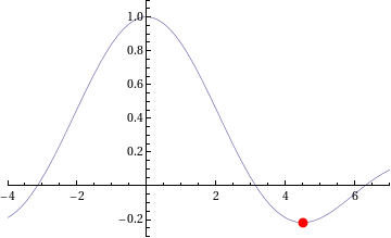
The example Python code I am going to give will solve a very simple local optimisation problem – The minimisation of the function sin(x)/x in the range [3.5,5.0] or, put another way, what are the x and y values of the centre of the red dot in the picture below.
The NAG/Python code to do this is given below (or you can download it here).
#!/usr/bin/env python
#Example 4 using NAG C library and ctypes - e04abc
#Mike Croucher - April 2008
#Concepts : Communication callback functions that use the C prototype void funct(double, double *,Nag_comm *)
from ctypes import *
from math import *
libnag = cdll.LoadLibrary("/opt/NAG/cllux08dgl/lib/libnagc_nag.so.8")
e04abc = libnag.e04abc
e04abc.restype=None
class Nag_Comm(Structure):
	_fields_ = [("flag", c_int),
                ("first", c_int),
 		("last", c_int),
		("nf",c_int),
		("it_prt",c_int),
		("it_maj_prt",c_int),
		("sol_sqp_prt",c_int),
		("sol_prt",c_int),
		("rootnode_sol_prt",c_int),
		("node_prt",c_int),
		("rootnode_prt",c_int),
		("g_prt",c_int),
		("new_lm",c_int),
		("needf",c_int),
		("p",c_void_p),
		("iuser",POINTER(c_int) ),
		("user",POINTER(c_double) ),
		("nag_w",POINTER(c_double) ),
		("nag_iw",POINTER(c_int) ),
		("nag_p",c_void_p),
		("nag_print_w",POINTER(c_double) ),
		("nag_print_iw",POINTER(c_int) ),
		("nrealloc",c_int)
		]
#define python objective function
def py_obj_func(x,ans,comm):
  ans[0] = sin(x) / x
  return
#create the type for the c callback function
C_FUNC = CFUNCTYPE(None,c_double,POINTER(c_double),POINTER(Nag_Comm))
#now create the c callback function
c_func = C_FUNC(py_obj_func)
#Set up the problem parameters
comm = Nag_Comm()
#e1 and e2 control the solution accuracy.  Setting them to 0 chooses the default values.
#See the documentation for e04abc for more details
e1 = c_double(0.0)
e2 = c_double(0.0)
#a and b define our starting interval
a = c_double(3.5)
b = c_double(5.0)
#xt will contain the x value of the minimum
xt=c_double(0.0)
#f will contain the function value at the minimum
f=c_double(0.0)
#max_fun is the maximum number of function evaluations we will allow
max_fun=c_int(100)
#Yet again I cheat for fail parameter.
fail=c_long(0)
e04abc(c_func,e1,e2,byref(a),byref(b),max_fun,byref(xt),byref(f),byref(comm),fail)
print "The minimum is in the interval  [%s,%s]" %(a.value,b.value)
print "The estimated result = %s" % xt.value
print "The function value at the minimum is %s " % f.value
print "%s evaluations were required" % comm.nf
If you run this code then you should get the following output
The minimum is in the interval  [4.4934093959,4.49340951173]
The estimated result = 4.49340945381
The function value at the minimum is -0.217233628211
10 evaluations were required
IFAIL oddness
My original version of this code used the trick of setting the NAG IFAIL parameter to c_int(0) to save me from worrying about the NagError structure (this is first explained in part 1) but when this example was tested it didn’t work on 64bit machines although it worked just fine on 32bit machines. Changing it to c_long(0) (as I have done in this example) made it work on both 32 and 64bit machines.
What I find odd is that in all my previous examples, c_int(0) worked just fine on both architectures. Eventually I will cover how to use the IFAIL parameter ‘properly’ but for now it is sufficient to be aware of this issue.
Scary Structures
Although this is the longest piece of code we have seen so far in this series, it contains no new Python/ctypes techniques at all. The only major difficulty I faced when writing it for the first time was making sure that I got the specification of the Nag_Comm structure correct by carefully working though the C specification of it in the nag_types.h file (included with the NAG C library installation) and transposing it to Python.
One of the biggest hurdles you will face when working with the NAG C library and Python is getting these structure definitions correct and some of them are truly HUGE. If you can get away with it then you are advised to copy and paste someone else’s definitions rather than create your own from scratch. In a later part of this series I will be releasing a Python module called PyNAG which will predefine some of the more common structures for you.
Callback functions with Communication
The objective function (that is, the function we want to minimise) is implemented as a callback function but it is a bit more complicated than the one we saw in part 3. This NAG routine expects the C prototype of your objective function to look like this:
void funct(double xc, double *fc, Nag_Comm *comm)
- xc is an input argument and is the point at which the value of f(x) is required.
- fc is an output argument and is the value of the function f at the current point x. Note that it is a pointer to double.
- Is a pointer to a structure of type Nag_Comm. Your function may or may not use this directly but the NAG routine almost certainly will. It is through this structure that the NAG routine can communicate various things to and from your function as and when is necessary.
so our C-types function prototype looks like this
C_FUNC = CFUNCTYPE(None,c_double,POINTER(c_double),POINTER(Nag_Comm))
whereas the python function itself is
#define python objective function
def py_obj_func(x,ans,comm):
  ans[0] = sin(x) / x
  return
Note that we need to do
ans[0] = sin(x) / x
rather than simply
ans = sin(x) / x
since ans is a pointer to double rather than just a double.
In this particular example I have only used the simplest feature provided by the Nag_Comm structure and that is to ask it how many times the objective function was called.
print "%s evaluations were required" % comm.nf
That’s it for this part of the series. Next time I’ll be looking at a more advanced optimisation routine. Feel free to post any comments, questions or suggestions.
This is part 4 of a series of articles devoted to demonstrating how to call the Numerical Algorithms Group (NAG) C library from Python. Click here for the index to this series.
The NAG C library makes extensive use of C structures throughout its code base and so we will need to know how to represent them in Python. For example, the NAG routine d01ajc is a general purpose one dimensional numerical integrator and one of it’s arguments is a structure called Nag_QuadProgress with the following prototype (found in the nag_types.h file that comes with the NAG C library)
  typedef struct
  {
    Integer num_subint;
    Integer fun_count;
    double *sub_int_beg_pts;
    double *sub_int_end_pts;
    double *sub_int_result;
    double *sub_int_error;
  } Nag_QuadProgress;
following the ctypes documentation on Structures and Unions, I came up with the following Python representation of this structure and it seems to work just fine.
class Nag_QuadProgress(Structure):
    _fields_ = [("num_subint", c_int),
                ("funcount", c_int),
		("sub_int_beg_pts",POINTER(c_double) ),
                ("sub_int_end_pts",POINTER(c_double)),
		("sub_int_result",POINTER(c_double)  ),
		("sub_int_error",POINTER(c_double)  )
		]
This is the only extra information we need in order to write a Python program that calculates the numerical approximation to an integral using the NAG routine d01ajc. Let’s calculate the integral of the function 4/(1.0+x*x) over the interval [0,1]. The code is as follows:
#!/usr/bin/env python
#Example 3 using NAG C library and ctypes
#d01ajc - one dimensional quadrature
#Mike Croucher - April 2008
#Concept introduced : Creating and using Python versions of structures such as Nag_QuadProgress
from ctypes import *
libnag = cdll.LoadLibrary("/opt/NAG/cllux08dgl/lib/libnagc_nag.so.8")

d01ajc = libnag.d01ajc
d01ajc.restype=None

class Nag_QuadProgress(Structure):
    _fields_ = [("num_subint", c_int),
                ("funcount", c_int),
		("sub_int_beg_pts",POINTER(c_double) ),
                ("sub_int_end_pts",POINTER(c_double)),
		("sub_int_result",POINTER(c_double)  ),
		("sub_int_error",POINTER(c_double)  )
		]

#define python function
def py_func(x):
	return 4./(1.0+x*x)

#create the prototype for the c callback function
C_FUNC = CFUNCTYPE(c_double,c_double )

#now create the c callback function
c_func = C_FUNC(py_func)

#set up the problem
a = c_double(0.0)
b = c_double(1.0)
nlimit = c_int(100)
epsr = c_double(0.00001)
ifail = c_int(0)

max_num_subint=c_int(200)
nlimit = c_int(0)
result=c_double(0.0)
epsabs= c_double(0.0)
epsrel=c_double(0.0001);
abserr=c_double(0.0);
qp=Nag_QuadProgress()

d01ajc(c_func,a,b,epsabs,epsrel,max_num_subint,byref(result) ,byref(abserr),byref(qp),ifail )
print "Approximation of integral= %s" %(result.value)
print "Number of function evaluations=%s" % qp.funcount
print "Number of subintervals used= %s" % qp.num_subint
Copy and paste (or download) this to a file called d01ajc.py, make it executable and run it by typing the following at a bash prompt.
chmod +x ./d01ajc.py

./d01ajc.py
If all has gone well then you should get following result
Approximation of integral= 3.14159265359
Number of function evaluations=21
Number of subintervals used= 1
Note that in order to create an instance of the Nag_QuadProgress structure I just do
qp=Nag_QuadProgress()
It is also useful to compare the C prototype of d01ajc
void nag_1d_quad_gen (double (*f)(double x),

double a, double b, double epsabs, double epsrel,

Integer max_num_subint, double *result, double *abserr,

Nag_QuadProgress *qp, NagError *fail)
with the way I called it in Python
d01ajc(c_func,a,b,epsabs,epsrel,max_num_subint,byref(result) ,byref(abserr),byref(qp),ifail )
Note how pointer arguments such as
double *abserr
are called as follows
byref(abserr)
Yet again I have cheated with the NagError parameter and just used c_int(0) instead of a proper NagError structure. NagError will be treated properly in a future article.
This is part 3 of a series of articles on how to use the NAG C Library with Python using the ctypes module. Click here for the introduction and index to the series.
Now that we have seen how to call the simplest of NAG functions from Python, it is time to move on and consider callback functions. If you don’t know what a callback function is then I think that the current version of the relevant Wikipedia article explains it well:
A callback is executable code that is passed as an argument to other code.
For example, say you want to want to find the zero of the function exp(-x)/x using a routine from the NAG library. Your first step would be to create a function that evaluates exp(-x)/x for any given x. You’ll later pass this function to the NAG routine to allow the routine to evaluate exp(-x)/x wherever it needs to.
Let’s take a look at some Python code that performs the calculation described above. The NAG routine I am using locates a zero of a continuous function in a given interval by a combination of the methods of linear interpolation, extrapolation and bisection and is called c05adc.
#!/usr/bin/env python

#Example 2 using NAG C libray and ctypes

#Mike Croucher - April 2008

#Concept Introduced : Callback functions
from ctypes import *

from math import *

libnag = cdll.LoadLibrary("/opt/NAG/cllux08dgl/lib/libnagc_nag.so.8")
c05adc = libnag.c05adc

c05adc.restype=None
#define python function
def py_func(x):
     return exp(-x)-x
#create the type for the c callback function

C_FUNC = CFUNCTYPE(c_double,c_double )
#now create the c callback function

c_func = C_FUNC(py_func)
a=c_double(0.0)

b=c_double(1.0)

xtol=c_double(0.00001)

ftol=c_double(0.0)

x=c_double(0.0)

fail=c_int(0)
c05adc(a, b, byref(x), c_func, xtol, ftol, fail );
print "result = %s" % (x.value)
Copy and paste (or download) this to a file called c05adc.py, make it executable and run it by typing the following at a bash prompt.
chmod +x ./c05adc.py

./c05adc.py
If all has gone well then you should get following output
result = 0.567143306605
Most of the code above will be familiar to anyone who worked through part 1 of this series. The first unfamiliar part might be
#define python function
def py_func(x):
     return exp(-x)-x
Which is nothing more than a standard Python function for calculating exp(-x)-x.
C_FUNC = CFUNCTYPE(c_double,c_double )
Here I have created a new C function prototype called C_FUNC by using the CFUNCTYPE function from the ctypes module. The general syntax of CFUNCTYPE is
CFUNCTYPE(return_type,input_arg1,input_arg2,input_arg3)
where the list of input arguments can be as long as you like. The C function I want to create from my Python function should return a c_double and have a single c_double input argument so I end up with CFUNCTYPE(c_double,c_double )
c_func = C_FUNC(py_func)
Here I have used the function prototype created earlier to generate a C function called c_func based on my Python function py_func.
c05adc(a, b, byref(x), c_func, xtol, ftol, fail );
Finally, I call the NAG routine c05adc using all of the arguments set up earlier. Note that I can pass my C function, c_func, to the NAG routine just as easily as I would any other argument. For reference, here is the original C prototype of the NAG routine along with a list of its arguments and what they mean
void nag_zero_cont_func_bd(double a, double b, double *x,

double (*f)(double x), double xtol,

double ftol, NagError *fail)
- a – (Input) The lower bound of the interval [a,b] in which the search for a zero will take place.
- b – (Input) The upper bound of the interval
- x – (Output) The approximation to the zero. Note that the C prototype uses a pointer to double and I have emulated this in python using the byref() function to pass x by reference.
- f – (Input) A pointer to the function who’s zeros we want to find. The C prototype might look complicated but, as you have seen, the implementation in Python is quite straightforward.
- xtol – (Input) The absolute tolerance to which the zero is required.
- ftol – (Input) a value such that if |f (x)| < ftol, x is accepted as the zero. ftol may be specified as0.0
- fail – The NAG error parameter. We haven’t covered structures yet so we can’t use NAGError properly but I have used the trick that the NAG routines will accept c_int(0) in order to accept the default error handling behaviour.
That’s it for now. Next time I will be looking at numerical integration using the NAG library which will require the introduction of structures.
As always, comments, queries and corrections are gratefully received.
This is part 2 of a series of articles devoted to demonstrating how to call the Numerical Algorithms Group (NAG) C library from Python. Click here for the index to this series.
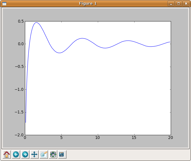
In part 1 I explained how to calculate the Cosine Integral, Ci(x), using Python and the NAG C library but the example code was a little dull in that it only calculated Ci(0.2). Before moving onto more advanced topics I thought it would be fun to use the python module, matplotlib, to generate a plot of the cosine integral.
#!/usr/bin/env python
from ctypes import *
import matplotlib.pyplot as plt

libnag = cdll.LoadLibrary("/opt/NAG/cllux08dgl/lib/libnagc_nag.so.8")
s13acc = libnag.s13acc
s13acc.restype=c_double

fail=c_int(0)
def nag_cos_integral(x):
	x=c_double(x)
	result= s13acc(x,fail)
	return result

xvals = [x*0.1 for x in range(1,200)]
yvals = map(nag_cos_integral,xvals)

plt.plot(xvals,yvals)
plt.show()
Click here to download this program – you’ll need a copy of the NAG C library to make it work. The output is shown below.
This is part 1 of a series of articles devoted to demonstrating how to call the Numerical Algorithms Group (NAG) C library from Python. Click here for the index to this series.
Our first NAG/Python example is going to use the NAG function s13acc which calculates the Cosine integral Ci(x) defined as

According to the NAG documentation, the algorithm used is based on several Chebyshev expansions. So, let’s see what we need to do to access this function from Python.
Assuming that you have installed the cllux08dgl implementation of the NAG C library, you should find that the following Python code evaluates Ci(x) for x=0.2.
#!/usr/bin/env python

from ctypes import *
libnag = cdll.LoadLibrary("/opt/NAG/cllux08dgl/lib/libnagc_nag.so.8")

nag_cos_integral = libnag.s13acc

nag_cos_integral.restype=c_double
x = c_double(0.2)

ifail=c_int(0)
y= nag_cos_integral( x, ifail )

print "x= %s, cos_integral= %s" % (x.value,y)
Save (or download) this to a file called s13acc.py, make it executable and run it by typing the following at a bash prompt.
chmod +x ./s13acc.py

./s13acc.py
If all has gone well then you should get following result
x= 0.2, cos_integral= -1.04220559567
Since this our first piece of NAG/Python code let’s go through it line by line.
from ctypes import *
This simply imports everything from the standard ctypes module and makes it available in the global namespace.
libnag = cdll.LoadLibrary("/opt/NAG/cllux08dgl/lib/libnagc_nag.so.8")

nag_cos_integral = libnag.s13acc
The first line loads the NAG library using the cldll.LoadLibrary() function and associates it with an object I have named libnag whereas the second line pulls the function s13acc out of libnag and associates it with an object having the more user-friendly name of nag_cos_integral.
This is the least portable part of the code. If you are using a different implementation of the NAG C library then you will need to change the path in the LoadLibrary function.
nag_cos_integral.restype=c_double
The ctypes module provides us with a set of C compatible data-types such as c_int, c_double, c_char and so on, and we have to use these when we interact with C functions. The object nag_cos_integral represents the NAG C function we wish to call and by default ctypes assumes that the return type of all C functions is of type c_int unless we tell it otherwise.
We know from the documentation for s13acc that its return type is double and so here we are using the restype method function to set the return type of nag_cos_integral to c_double.
x = c_double(0.2)

ifail=c_int(0)
Here, we are setting up our input arguments. x is straightforward enough but the observant reader will notice that there is something fishy going on with the ifail parameter. The NAG documentation tells us that the ifail parameter of s13acc should be a pointer to a NagError structure but structures are a complication that I don’t want to deal with here so I have cheated and used the fact that the integer 0 is defined as NAGERR_DEFAULT via an enumeration in the C library header file. In short, this means that I don’t have to use a NagError structure if I don’t want to. Full details can be found in section 2.6 of the Essential Introduction to the NAG C Library.
We’ll look at how to use the NagError structure properly via Python in a later article for those who need it.
y= nag_cos_integral( x, ifail )
Here we pass our input parameters to the nag_cos_integral function and store the result in y. When I was working all of this out for the first time, I expected y to be of type c_double. After all, we earlier used restype to set the return type of nag_cos_integral to c_double so that’s what I expected to get but it turns out that y is a plain old python double. This is clearly explained in the ctypes documentation and I quote the relevant section below
‘Fundamental data types, when returned as foreign function call results, or, for example, by retrieving structure field members or array items, are transparently converted to native Python types. In other words, if a foreign function has a restype of c_char_p, you will always receive a Python string, not a c_char_p instance.’
print "x= %s, cos_integral= %s" % (x.value,y)
Finally, we actually print the output. Since x is a c_double we need to use the value attribute to ensure that 0.2 gets printed rather than c_double(0.2). The variable y is a python double as explained earlier so it needs no special treatment.
That’s it for this article in the series. Next time I’ll give an example using this function along with matplotlib to produce some more interesting output before moving onto callback functions.
As always, questions and comments are welcomed.
The NAG library is possibly the most comprehensive numerical library available today with over 1500 functions and a long and distinguished history going back almost 40 years. Although it is commercial, NAG is a not-for-profit company and has donated large amounts of code to the open source community over the years. The library covers many application areas including special functions, optimization, curve fitting, statistics, numerical differentiation and linear algebra among others with even more coming up in the next release. It has been available in several different programming languages over the years but these days you can get it in essentially four flavours – The NAG Fortran Library, The NAG C Library, the Maple-NAG connector and the NAG Toolbox for MATLAB.
I have been supporting users of the NAG library at Manchester University for a few years now and one of the most common reactions I get from a potential user of the NAG libraries when they see the list of available languages is to say ‘I don’t program in any of those – I program in XYZ – so the NAG library is no use to me.’ where XYZ might be Java, Perl, Visual Basic, Python, R or one of any number of weird and wonderful possibilities.
It turns out that YOUR choice of language almost doesn’t matter as far as NAG is concerned since, with a bit of work, you can call the NAG routines from pretty much any language you care to mention. Put another way, NAG program in Fortran (and C) so you don’t have to. One language that has been mentioned a lot recently is Python.
Mat Cross, an employee of NAG, wrote a guide a little while ago giving detailed instructions on how to call the NAG Fortran library from Python using a module called F2PY and very nice it is too. However, some people are never happy and almost as soon as the article was published I started getting queries about the NAG C library and Python. As far as I could tell this particular combination hadn’t been covered by anyone before so I rolled up my sleeves to see what I could come up with.
After all, how hard could it be?
I have lost count of the number of times I have regretted uttering that particular phrase but in this case, thanks to a wonderful Python module called ctypes, the answer turns out to be ‘Not nearly as hard as you might expect’.
The results of my investigations will be posted on Walking Randomly over the next few weeks and will include several examples of how to use the NAG C library within Python. I’ll start off with the simplest of NAG functions and steadily move towards some of the most complex. On the way we will cover several areas of numerical mathematics including special functions, numerical quadrature, root finding and optimization.
I will initially be concentrating on Ubuntu Linux since that is my favourite development environment but I am aware that users of both NAG and Python make use of many platforms including Windows and Mac OS X. If there is sufficient interest then I will make other platform-specific articles available in the future.
The list below contains links to all of the articles published in the series so far and will be expanded as new ones come online so this post will eventually serve as an index to the whole series. Extra topics may be considered on request.
Topic List (will be expanded as new articles are available)
- Making simple NAG C functions available to Python
- Plotting the Cosine Integral using NAG and matplotlib
- Callback functions (The example code given is for finding the zero’s of an equation)
- Structures (The example code given is for Numerical Integration)
- Callback functions with communication (The example code solves a simple 1d minimization problem)
- PyNAG – A Python package for interfacing with the NAG C Library
Implementation specifics
The NAG C library is available for a wide range of platforms and C compilers (representing 26 different combinations when I last counted) but I only wanted to focus on one for the sake of sanity! In particular, I am using cllux08dgl throughout this series which is for 32bit Linux and was compiled using the gcc compiler. I am using version 8.10 of Ubuntu Linux.
I imagine that most of what I write will be directly transferable, with minor modifications, to other versions of the NAG C library. After all Python is quite portable but there may be some differences if you are using a platform wildly different from mine. Where I am able, I will help people get the examples working on their platform of choice but reserve the right to refer you to the NAG support team if necessary.
Finally, I have developed all of this series using 2.5.2 and have no idea if it will work in later versions or not.