
Archive for the ‘programming’ Category
A Mathematica user contacted me recently and asked why
(1/16 Cos[a] (Cos[b] + 15 Cos[3 b])) === (1/8 Cos[b] (-7 + 15 Cos[2b])Cos[a])
returned False when he expected True. Let’s take a look at what is going on here.
The SameQ command (===) and the Equal command (==) are subtly different. Equal (==) tests to see if two expressions are mathematically equivalent whereas SameQ tests to see if they are structurally equivalent. In general, SameQ is the stricter of the two tests and is often too strict for our needs.
A very simple example
The simplest example might be to compare 2 and 2. (That is 2 with a period at the end)
Mathematically these are the same since they both represent the number two. However, from a Mathematica structural point of view, they are different since one has infinite precision whereas the other has double precision. So, we have
2==2. gives True
2===2. gives False
A more complicated example
Sqrt[2] + Sqrt[3] == Sqrt[5 + 2 Sqrt[6]] which gives True
Sqrt[2] + Sqrt[3] === Sqrt[5 + 2 Sqrt[6]] which gives False
Mathematically the above is always true but the structure of the expressions on the LHS and RHS are different under normal evaluation rules.
So, what do I mean by ‘structurally equivalent?’. To be honest, I am slightly woolly on this myself but in my head I consider two expressions to be structurally equivalent if their TreeForms are the same
TreeForm[Sqrt[2] + Sqrt[3] ]
![TreeForm[Sqrt[2] + Sqrt[3] ]](https://www.walkingrandomly.com/images/mathematica8/treeform_lhs.png)
TreeForm[Sqrt[5 + 2 Sqrt[6]] ]
![TreeForm[Sqrt[5 + 2 Sqrt[6]] ]]](https://www.walkingrandomly.com/images/mathematica8/treeform_rhs.png)
The important thing to remember here is that the argument to TreeForm is evaluated by Mathematica before it gets passed to TreeForm. So, the above images show us that under normal evaluation rules, these two expressions have different structural forms. In the next example we’ll see how this detail can matter
Exp[I Pi] and all that
Let’s look at
Exp[I Pi] === -1
Would that be True or False based on what we have seen so far? It is certainly mathematically true but remember that a triple equals requires both sides to be structurally equivalent and at first sight it appears that this isn’t the case here. You might expect Exp[I Pi] to have a very different TreeForm from -1 and so you’d expect the above to evaluate to False. However if you do
TreeForm[Exp[I Pi]]
then you get a single box containing -1. This occurs because Mathematica evaluates Exp[I Pi] to -1 before passing to TreeForm. This evaluation also occurs when you do Exp[I Pi] === -1 so what you are really testing is -1===-1 which is obviously True.
Back to the original example
(1/16 Cos[a] (Cos[b] + 15 Cos[3 b])) === (1/8 Cos[b] (-7 + 15 Cos[2b])Cos[a])
If you use === then it returns False and this is ‘obviously’ the case because if you evaluate the TreeForms of both expressions then you’ll see that they get stored with different structural forms after being evaluated.
TreeForm[(1/16 Cos[a] (Cos[b] + 15 Cos[3 b]))]
![TreeForm[(1/16 Cos[a] (Cos[b] + 15 Cos[3 b]))]](https://www.walkingrandomly.com/images/mathematica8/treeform1_lhs.png)
TreeForm[(1/8 Cos[b] (-7 + 15 Cos[2 b]) Cos[a])]
![TreeForm[(1/8 Cos[b] (-7 + 15 Cos[2 b]) Cos[a])]]](https://www.walkingrandomly.com/images/mathematica8/treeform1_rhs.png)
Since we are interested in mathematical equivalence, however, we use ==
(1/16 Cos[a] (Cos[b] + 15 Cos[3 b])) == (1/8 Cos[b] (-7 + 15 Cos[2 b]) Cos[a])
What happens this time, however, is that Mathematica returns the original expression unevaluated. This is because, under the standard set of transformations that Mathematica applies when it evaluates ==, it can’t be sure one way or the other and so it gives up.
To proceed we wrap the whole thing in FullSimplify which essentially says to Mathematica ‘Use everything you’ve got to try and figure this out – no matter how long it takes’ I.e. you allow it to use more transforms.
FullSimplify[(1/16 Cos[a] (Cos[b] + 15 Cos[3 b])) == (1/8 Cos[b] (-7 + 15 Cos[2 b]) Cos[a])]

True
Finally, we have the result that the user expected.
Someone recently contacted me with a problem – she wanted to use MATLAB to perform a weighted quadratic curve fit to a set of data. Now, if she had the curve fitting toolbox this would be nice and easy:
x=[ 1 2 3 4 5];
y=[1.4 2.2 3.5 4.9 2.3];
w=[1 1 1 1 0.1];

f=fittype('poly2');
options=fitoptions('poly2');
options.Weights=[1 1 1 1 0.1];
fun=fit(x',y',f,options);
p1=fun.p1;
p2=fun.p2;
p3=fun.p3;

myfit = [p1 p2 p3]

myfit =
   -0.1599    1.8554   -0.5014
So, our weighted quadratic curve fit is y = -0.4786*x^2 + 3.3214*x – 1.84
So far so good but she didn’t have access to the curve fitting toolbox so what to do? One function that almost meets her needs is the standard MATLAB function polyfit which can do everything apart from the weighted part.
polyfit(x,y,2)
ans =
   -0.4786    3.3214   -1.8400
which would agree with the curve fitting toolbox if we set the weights to all ones. Sadly, however, we cannot supply the weights to the polyfit function as it currently stands (as of 2010b). My solution was to create a new function, wpolyfit, that does accept a vector of weights:
wpolyfit(x,y,2,w)
ans =
   -0.1599    1.8554   -0.5014
So where is this new function I hear you ask? Normally this is where I would provide you with a download link but unfortunately I created wpolyfit by making a very small modification to the original built-in polyfit function and so I might be on dicey ground by distributing it. So, instead I will give you instructions on how to make it yourself. I did this using MATLAB 2010b but it should work with other versions assuming that the polyfit function hasn’t changed much.
First, open up the polyfit function in the MATLAB editor
edit polyfit
change the first line so that it reads
function [p,S,mu] = wpolyfit(x,y,n,w)
Now, just before the line that reads
% Solve least squares problem.
add the following
w=sqrt(w(:));
y=y.*w;
for j=1:n+1
    V(:,j) = w.*V(:,j);
end
Save the file as wpolyfit.m and you are done. I won’t go over the theory of how this works because it is covered very nicely here. Comments welcomed.
If you love your code…set it free! That’s what Will Robertson did when he released the first version of colorbarplot for Mathematica. I liked what he did but it didn’t do quite enough for my needs so I added some stuff to it and a new version was born.
Our package starting getting users and some of those users asked for things so Will and I added yet more stuff and colorbarplot version 0.5 was born.
Finally, one of those users, Thomas Zell of the University of Cologne, has added more functionality of his own resulting in version 0.6 of colorbarplot. So, what’s new?
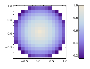
Well, if you have data in the form of a two-dimensional array, in which not every entry has valid numerical data, the following will now work without error:
set1 = Table[
   If[Sqrt[x^2 + y^2] < 1, Sqrt[1 - Sqrt[x^2 + y^2]]], {x, -1, 1,      0.125}, {y, -1, 1, 0.125}];
ColorbarPlot[set1, InterpolationOrder -> 0,
 DataRange -> {{-1, 1}, {-1, 1}}]
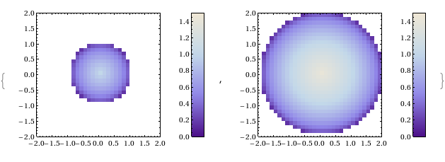
Next up, if you want to compare two data sets, the plots have to have the same scale even if the data sets have different sizes. This can now be achieved with the PlotRange option:
set2 = Table[
  If[Sqrt[x^2 + y^2] < 2, Sqrt[2 - Sqrt[x^2 + y^2]]], {x, -2, 2,    0.125}, {y, -2, 2, 0.125}];

{ColorbarPlot[set1, InterpolationOrder -> 0,
 DataRange -> {{-1, 1}, {-1, 1}},
 PlotRange -> {{-2, 2}, {-2, 2}, {0, 1.5}}],
ColorbarPlot[set2, InterpolationOrder -> 0,
 DataRange -> {{-2, 2}, {-2, 2}},
 PlotRange -> {{-2, 2}, {-2, 2}, {0, 1.5}}]}
This is great stuff, helps make colorbarplot more useful and turns the package into a truly international collaboration ;)
- ColorbarPlot’s github page The latest version will always be available here
- ColorbarPlot’s page in the Wolfram Library This is often out of date.
- ColorbarPlot 0.6 from the WalkingRandomly server
- ColorbatPlot 0.5 My write up of a previous version
- ColorbarPlot 0.4 My write up of a previous version
- ColorbarPlot 0.3 My write up of a previous version
Have you published anything that uses colorbarplot?
If you have published anything that uses our little package then please do let us know. We know we have users so it would be great to see how you are using it. The more feedback we get, the more likely we are to want to develop it further.
Some time ago now, Sam Shah of Continuous Everywhere but Differentiable Nowhere fame discussed the standard method of obtaining the square root of the imaginary unit, i, and in the ensuing discussion thread someone asked the question “What is i^i – that is what is i to the power i?”
Sam immediately came back with the answer e^(-pi/2) = 0.207879…. which is one of the answers but as pointed out by one of his readers, Adam Glesser, this is just one of the infinite number of potential answers that all have the form e^{-(2k+1) pi/2} where k is an integer. Sam’s answer is the principle value of i^i (incidentally this is the value returned by google calculator if you google i^i – It is also the value returned by Mathematica and MATLAB). Life gets a lot more complicated when you move to the complex plane but it also gets a lot more interesting too.
While on the train into work one morning I was thinking about Sam’s blog post and wondered what the principal value of i^i^i (i to the power i to the power i) was equal to. Mathematica quickly provided the answer:
N[I^I^I]
0.947159+0.320764 I
So i is imaginary, i^i is real and i^i^i is imaginary again. Would i^i^i^i be real I wondered – would be fun if it was. Let’s see:
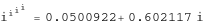
N[I^I^I^I]
0.0500922+0.602117 I
gah – a conjecture bites the dust – although if I am being honest it wasn’t a very good one. Still, since I have started making ‘power towers’ I may as well continue and see what I can see. Why am I calling them power towers? Well, the calculation above could be written as follows:
As I add more and more powers, the left hand side of the equation will tower up the page….Power Towers. We now have a sequence of the first four power towers of i:
i = i
i^i = 0.207879
i^i^i = 0.947159 + 0.32076 I
i^i^i^i = 0.0500922+0.602117 I
Sequences of power towers
“Will this sequence converge or diverge?”, I wondered. I wasn’t in the mood to think about a rigorous mathematical proof, I just wanted to play so I turned back to Mathematica. First things first, I needed to come up with a way of making an arbitrarily large power tower without having to do a lot of typing. Mathematica’s Nest function came to the rescue and the following function allows you to create a power tower of any size for any number, not just i.
tower[base_, size_] := Nest[N[(base^#)] &, base, size]
Now I can find the first term of my series by doing
In[1]:= tower[I, 0]

Out[1]= I
Or the 5th term by doing
In[2]:= tower[I, 4]

Out[2]= 0.387166 + 0.0305271 I
To investigate convergence I needed to create a table of these. Maybe the first 100 towers would do:
ColumnForm[
 Table[tower[I, n], {n, 1, 100}]
 ]
The last few values given by the command above are
0.438272+ 0.360595 I
0.438287+ 0.360583 I
0.438287+ 0.3606 I
0.438275+ 0.360591 I
0.438289+ 0.360588 I
Now this is interesting – As I increased the size of the power tower, the result seemed to be converging to around 0.438 + 0.361 i. Further investigation confirms that the sequence of power towers of i converges to 0.438283+ 0.360592 i. If you were to ask me to guess what I thought would happen with large power towers like this then I would expect them to do one of three things – diverge to infinity, stay at 1 forever or quickly converge to 0 so this is unexpected behaviour (unexpected to me at least).
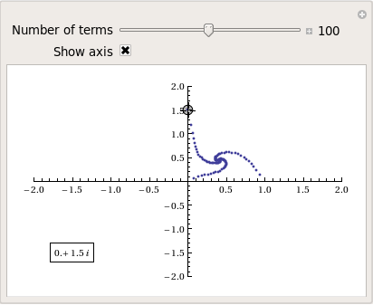
They converge, but how?
My next thought was ‘How does it converge to this value? In other words, ‘What path through the complex plane does this sequence of power towers take?” Time for a graph:
tower[base_, size_] := Nest[N[(base^#)] &, base, size];
complexSplit[x_] := {Re[x], Im[x]};
ListPlot[Map[complexSplit, Table[tower[I, n], {n, 0, 49, 1}]],
 PlotRange -> All]
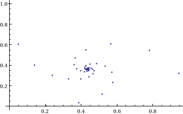
Who would have thought you could get a spiral from power towers? Very nice! So the next question is ‘What would happen if I took a different complex number as my starting point?’ For example – would power towers of (0.5 + i) converge?’
The answer turns out to be yes – power towers of (0.5 + I) converge to 0.541199+ 0.40681 I but the resulting spiral looks rather different from the one above.
tower[base_, size_] := Nest[N[(base^#)] &, base, size];
complexSplit[x_] := {Re[x], Im[x]};
ListPlot[Map[complexSplit, Table[tower[0.5 + I, n], {n, 0, 49, 1}]],
 PlotRange -> All]
 The zoo of power tower spirals
So, taking power towers of two different complex numbers results in two qualitatively different ‘convergence spirals’. I wondered how many different spiral types I might find if I consider the entire complex plane? I already have all of the machinery I need to perform such an investigation but investigation is much more fun if it is interactive. Time for a Manipulate
complexSplit[x_] := {Re[x], Im[x]};

tower[base_, size_] := Nest[N[(base^#)] &, base, size];

generatePowerSpiral[p_, nmax_] :=
  Map[complexSplit, Table[tower[p, n], {n, 0, nmax-1, 1}]];

Manipulate[const = p[[1]] + p[[2]] I;
 ListPlot[generatePowerSpiral[const, n],
 PlotRange -> {{-2, 2}, {-2, 2}}, Axes -> ax,
 Epilog -> Inset[Framed[const], {-1.5, -1.5}]], {{n, 100,
 "Number of terms"}, 1, 200, 1,
 Appearance -> "Labeled"}, {{ax, True, "Show axis"}, {True,
 False}}, {{p, {0, 1.5}}, Locator}]
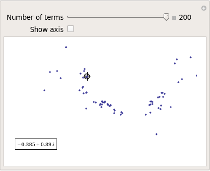
After playing around with this Manipulate for a few seconds it became clear to me that there is quite a rich diversity of these convergence spirals. Here are a couple more
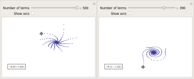
Some of them take a lot longer to converge than others and then there are those that don’t converge at all:
Optimising the code a little
Before I could investigate convergence any further, I had a problem to solve: Sometimes the Manipulate would completely freeze and a message eventually popped up saying “One or more dynamic objects are taking excessively long to finish evaluating……” What was causing this I wondered?
Well, some values give overflow errors:
In[12]:= generatePowerSpiral[-1 + -0.5 I, 200]

General::ovfl: Overflow occurred in computation. >>
General::ovfl: Overflow occurred in computation. >>
General::ovfl: Overflow occurred in computation. >>
General::stop: Further output of General::ovfl will be suppressed during this calculation. >>
Could errors such as this be making my Manipulate unstable? Let’s see how long it takes Mathematica to deal with the example above
AbsoluteTiming[ListPlot[generatePowerSpiral[-1 -0.5 I, 200]]]
On my machine, the above command typically takes around 0.08 seconds to complete compared to 0.04 seconds for a tower that converges nicely; it’s slower but not so slow that it should break Manipulate. Still, let’s fix it anyway.
Look at the sequence of values that make up this problematic power tower
generatePowerSpiral[-0.8 + 0.1 I, 10]

{{-0.8, 0.1}, {-0.668442, -0.570216}, {-2.0495, -6.11826},
{2.47539*10^7,1.59867*10^8}, {2.068155430437682*10^-211800874,
-9.83350984373519*10^-211800875}, {Overflow[], 0}, {Indeterminate,
  Indeterminate}, {Indeterminate, Indeterminate}, {Indeterminate,
  Indeterminate}, {Indeterminate, Indeterminate}}
Everything is just fine until the term {Overflow[],0} is reached; after which we are just wasting time. Recall that the functions I am using to create these sequences are
complexSplit[x_] := {Re[x], Im[x]};
tower[base_, size_] := Nest[N[(base^#)] &, base, size];
generatePowerSpiral[p_, nmax_] :=
  Map[complexSplit, Table[tower[p, n], {n, 0, nmax-1, 1}]];
The first thing I need to do is break out of tower’s Nest function as soon as the result stops being a complex number and the NestWhile function allows me to do this. So, I could redefine the tower function to be
tower[base_, size_] :=
 NestWhile[N[(base^#)] &, base, MatchQ[#, _Complex] &, 1, size]
However, I can do much better than that since my code so far is massively inefficient. Say I already have the first n terms of a tower sequence; to get the (n+1)th term all I need to do is a single power operation but my code is starting from the beginning and doing n power operations instead. So, to get the 5th term, for example, my code does this
I^I^I^I^I
instead of
(4th term)^I
The function I need to turn to is yet another variant of Nest – NestWhileList
fasttowerspiral[base_, size_] :=
 Quiet[Map[complexSplit,
 NestWhileList[N[(base^#)] &, base, MatchQ[#, _Complex] &, 1,
 size, -1]]];
The Quiet function is there to prevent Mathematica from warning me about the Overflow error. I could probably do better than this and catch the Overflow error coming before it happens but since I’m only mucking around, I’ll leave that to an interested reader. For now it’s enough for me to know that the code is much faster than before:
(*Original Function*)
AbsoluteTiming[generatePowerSpiral[I, 200];]

{0.036254, Null}
(*Improved Function*)
AbsoluteTiming[fasttowerspiral[I, 200];]

{0.001740, Null}
A factor of 20 will do nicely!
Making Mathematica faster by making it stupid
I’m still not done though. Even with these optimisations, it can take a massive amount of time to compute some of these power tower spirals. For example
spiral = fasttowerspiral[-0.77 - 0.11 I, 100];
takes 10 seconds on my machine which is thousands of times slower than most towers take to compute. What on earth is going on? Let’s look at the first few numbers to see if we can find any clues
In[34]:= spiral[[1 ;; 10]]

Out[34]= {{-0.77, -0.11}, {-0.605189, 0.62837}, {-0.66393,
  7.63862}, {1.05327*10^10,
  7.62636*10^8}, {1.716487392960862*10^-155829929,
  2.965988537183398*10^-155829929}, {1., \
-5.894184073663391*10^-155829929}, {-0.77, -0.11}, {-0.605189,
  0.62837}, {-0.66393, 7.63862}, {1.05327*10^10, 7.62636*10^8}}
The first pair that jumps out at me is {1.71648739296086210^-155829929, 2.96598853718339810^-155829929} which is so close to {0,0} that it’s not even funny! So close, in fact, that they are not even double precision numbers any more. Mathematica has realised that the calculation was going to underflow and so it caught it and returned the result in arbitrary precision.
Arbitrary precision calculations are MUCH slower than double precision ones and this is why this particular calculation takes so long. Mathematica is being very clever but its cleverness is costing me a great deal of time and not adding much to the calculation in this case. I reckon that I want Mathematica to be stupid this time and so I’ll turn off its underflow safety net.
SetSystemOptions["CatchMachineUnderflow" -> False]
Now our problematic calculation takes 0.000842 seconds rather than 10 seconds which is so much faster that it borders on the astonishing. The results seem just fine too!
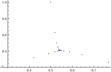
When do the power towers converge?
We have seen that some towers converge while others do not. Let S be the set of complex numbers which lead to convergent power towers. What might S look like? To determine that I have to come up with a function that answers the question ‘For a given complex number z, does the infinite power tower converge?’ The following is a quick stab at such a function
convergeQ[base_, size_] :=
  If[Length[
     Quiet[NestWhileList[N[(base^#)] &, base, Abs[#1 - #2] > 0.01 &,
       2, size, -1]]] < size, 1, 0];
The tolerance I have chosen, 0.01, might be a little too large but these towers can take ages to converge and I’m more interested in speed than accuracy right now so 0.01 it is. convergeQ returns 1 when the tower seems to converge in at most size steps and 0 otherwise.:
In[3]:= convergeQ[I, 50]
Out[3]= 1

In[4]:= convergeQ[-1 + 2 I, 50]
Out[4]= 0
So, let’s apply this to a section of the complex plane.
towerFract[xmin_, xmax_, ymin_, ymax_, step_] :=
 ArrayPlot[
 Table[convergeQ[x + I y, 50], {y, ymin, ymax, step}, {x, xmin, xmax,step}]]
towerFract[-2, 2, -2, 2, 0.1]
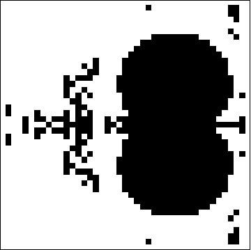
That looks like it might be interesting, possibly even fractal, behaviour but I need to increase the resolution and maybe widen the range to see what’s really going on. That’s going to take quite a bit of calculation time so I need to optimise some more.
Going Parallel
There is no point in having machines with two, four or more processor cores if you only ever use one and so it is time to see if we can get our other cores in on the act.
It turns out that this calculation is an example of a so-called embarrassingly parallel problem and so life is going to be particularly easy for us. Basically, all we need to do is to give each core its own bit of the complex plane to work on, collect the results at the end and reap the increase in speed. Here’s the full parallel version of the power tower fractal code
(*Complete Parallel version of the power tower fractal code*)

convergeQ[base_, size_] :=
 If[Length[
 Quiet[NestWhileList[N[(base^#)] &, base, Abs[#1 - #2] > 0.01 &,
 2, size, -1]]] < size, 1, 0];

LaunchKernels[];
DistributeDefinitions[convergeQ];
ParallelEvaluate[SetSystemOptions["CatchMachineUnderflow" -> False]];

towerFractParallel[xmin_, xmax_, ymin_, ymax_, step_] :=
 ArrayPlot[
 ParallelTable[
 convergeQ[x + I y, 50], {y, ymin, ymax, step}, {x, xmin, xmax, step}
, Method -> "CoarsestGrained"]]
This code is pretty similar to the single processor version so let’s focus on the parallel modifications. My convergeQ function is no different to the serial version so nothing new to talk about there. So, the first new code is
LaunchKernels[];
This launches a set of parallel Mathematica kernels. The amount that actually get launched depends on the number of cores on your machine. So, on my dual core laptop I get 2 and on my quad core desktop I get 4.
DistributeDefinitions[convergeQ];
All of those parallel kernels are completely clean in that they don’t know about my user defined convergeQ function. This line sends the definition of convergeQ to all of the freshly launched parallel kernels.
ParallelEvaluate[SetSystemOptions["CatchMachineUnderflow" -> False]];
Here we turn off Mathematica’s machine underflow safety net on all of our parallel kernels using the ParallelEvaluate function.
That’s all that is necessary to set up the parallel environment. All that remains is to change Map to ParallelMap and to add the argument Method -> “CoarsestGrained” which basically says to Mathematica ‘Each sub-calculation will take a tiny amount of time to perform so you may as well send each core lots to do at once’ (click here for a blog post of mine where this is discussed further).
That’s all it took to take this embarrassingly parallel problem from a serial calculation to a parallel one. Let’s see if it worked. The test machine for what follows contains a T5800 Intel Core 2 Duo CPU running at 2Ghz on Ubuntu (if you want to repeat these timings then I suggest you read this blog post first or you may find the parallel version going slower than the serial one). I’ve suppressed the output of the graphic since I only want to time calculation and not rendering time.
(*Serial version*)
In[3]= AbsoluteTiming[towerFract[-2, 2, -2, 2, 0.1];]
Out[3]= {0.672976, Null}

(*Parallel version*)
In[4]= AbsoluteTiming[towerFractParallel[-2, 2, -2, 2, 0.1];]
Out[4]= {0.532504, Null}

In[5]= speedup = 0.672976/0.532504
Out[5]= 1.2638
I was hoping for a bit more than a factor of 1.26 but that’s the way it goes with parallel programming sometimes. The speedup factor gets a bit higher if you increase the size of the problem though. Let’s increase the problem size by a factor of 100.
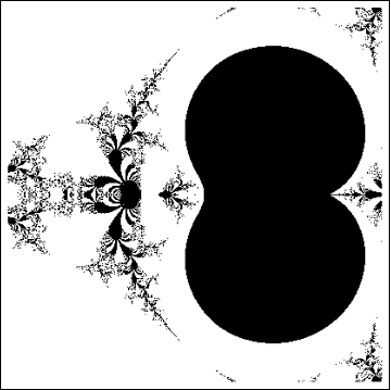
towerFractParallel[-2, 2, -2, 2, 0.01]
The above calculation took 41.99 seconds compared to 63.58 seconds for the serial version resulting in a speedup factor of around 1.5 (or about 34% depending on how you want to look at it).
Other optimisations
I guess if I were really serious about optimising this problem then I could take advantage of the symmetry along the x axis or maybe I could utilise the fact that if one point in a convergence spiral converges then it follows that they all do. Maybe there are more intelligent ways to test for convergence or maybe I’d get a big speed increase from programming in C or F#? If anyone is interested in having a go at improving any of this and succeeds then let me know.
I’m not going to pursue any of these or any other optimisations, however, since the above exploration is what I achieved in a single train journey to work (The write-up took rather longer though). I didn’t know where I was going and I only worried about optimisation when I had to. At each step of the way the code was fast enough to ensure that I could interact with the problem at hand.
Being mostly ‘fast enough’ with minimal programming effort is one of the reasons I like playing with Mathematica when doing explorations such as this.
Treading where people have gone before
So, back to the power tower story. As I mentioned earlier, I did most of the above in a single train journey and I didn’t have access to the internet. I was quite excited that I had found a fractal from such a relatively simple system and very much felt like I had discovered something for myself. Would this lead to something that was publishable I wondered?
Sadly not!
It turns out that power towers have been thoroughly investigated and the act of forming a tower is called tetration. I learned that when a tower converges there is an analytical formula that gives what it will converge to:

Where W is the Lambert W function (click here for a cool poster for this function). I discovered that other people had already made Wolfram Demonstrations for power towers too
There is even a website called tetration.org that shows ‘my’ fractal in glorious technicolor. Nothing new under the sun eh?
Parting shots
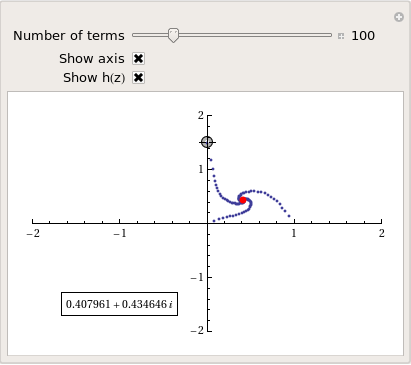
Well, I didn’t discover anything new but I had a bit of fun along the way. Here’s the final Manipulate I came up with
Manipulate[const = p[[1]] + p[[2]] I;
 If[hz,
  ListPlot[fasttowerspiral[const, n], PlotRange -> {{-2, 2}, {-2, 2}},
    Axes -> ax,
   Epilog -> {{PointSize[Large], Red,
      Point[complexSplit[N[h[const]]]]}, {Inset[
       Framed[N[h[const]]], {-1, -1.5}]}}]
  , ListPlot[fasttowerspiral[const, n],
   PlotRange -> {{-2, 2}, {-2, 2}}, Axes -> ax]
  ]
 , {{n, 100, "Number of terms"}, 1, 500, 1, Appearance -> "Labeled"}
 , {{ax, True, "Show axis"}, {True, False}}
 , {{hz, True, "Show h(z)"}, {True, False}}
 , {{p, {0, 1.5}}, Locator}
 , Initialization :> (
   SetSystemOptions["CatchMachineUnderflow" -> False];
   complexSplit[x_] := {Re[x], Im[x]};
   fasttowerspiral[base_, size_] :=
    Quiet[Map[complexSplit,
      NestWhileList[N[(base^#)] &, base, MatchQ[#, _Complex] &, 1,
       size, -1]]];
   h[z_] := -ProductLog[-Log[z]]/Log[z];
   )
 ]
and here’s a video of a zoom into the tetration fractal that I made using spare cycles on Manchester University’s condor pool.
If you liked this blog post then you may also enjoy:
Because I spend so much time talking about and helping people with MATLAB, I often get asked to recommend a good MATLAB book. I actually find this a rather difficult question to answer because, contrary to what people seem to expect, I have a relatively small library of MATLAB books.
However, one could argue the fact that I only have a small library of books suggests that I hit upon the good ones straight away. So, for those in the market for an introductory MATLAB book, here are my recommendations
MATLAB Guide by Desmond and Nicholas Higham

If you only ever buy one MATLAB book then this should be it. It starts off with a relatively fast paced mini-tutorial that could be considered a sight-seeing tour of MATLAB and its functionality. Once this is done, the authors get down to the business of teaching you the fundamentals of MATLAB in a systematic,thorough and enjoyable manner.
Unlike some books I have seen, this one doesn’t just show you MATLAB syntax; instead it shows you how to be a good MATLAB programmer from the beginning. Your programs will be efficient, robust and well documented because you will know how to leverage MATLAB’s particular strengths.
One aspect of the Higham’s book that I particularly like is that they include many mathematical examples that are intrinsically interesting in their own right. This was where I first learned of Maurer roses, Viswanath’s constant and eigenvalue roulette for example. Systems such as MATLAB are ideal for demonstrating cool little mathematical ideas and so it’s great to see so many of them sprinkled throughout an introductory textbook such as this one.
The only downside to the current edition is that the chapter on the symbolic toolbox is out of date since it refers to the old Maple based one rather than the current Mupad based system (See my post here for more details on this transition). This is only a minor gripe, however, and I only really mention it at all in an attempt to give a review that looks more balanced.
Full disclosure: One of the authors, Nicholas Higham, works at the same university as me. However, we are in different departments and I paid for my own copy of his book in full.
MATLAB: A Practical Introduction to Programming and Problem Solving by Stormy Attaway

I haven’t had this book as long as I’ve had the Higham book and I haven’t even completely finished it yet. I am, however, very impressed with it (as an aside, it’s also the first technical book I ever bought using the iPad and Android Kindle apps).
One of the key things that I like most about this one is that the text is liberally sprinkled with ‘Quick Questions’ that give you a little scenario and ask you how you’d deal with it in MATLAB. This is quickly followed by a model answer that explains the concepts. These help break up the text, make you stop and think and ultimately lead to you thinking in a more MATLABy way. There is also a good amount of exercises at the end of each chapter (no model solutions provided though).
The book is split into two main parts with the first half concentrating on MATLAB fundamentals such as matrices, vectorization, strings, functions etc while the second half covers mathematical applications such as statistics, curve fitting and numerical integration. So, it’ll take you from being a complete novice to someone who knows their way around a reasonable portion of the system.
Since I first bought this book using the Kindle app on my iPad I thought I’d quickly mention how that worked out for me. In short, I hated the Kindle presentation so much that I went out and bought the physical version of the book as well. The paper version is beautifully formatted and presented whereas the Kindle version is just awful. It’s hard to navigate, looks awful and basically makes one wish that they had just given you a pdf file instead!
Not long after publishing my article, A faster version of MATLAB’s fsolve using the NAG Toolbox for MATLAB, I was contacted by Biao Guo of Quantitative Finance Collector who asked me what I could do with the following piece of code.
function MarkowitzWeight = fsolve_markowitz_MATLAB()

RandStream.setDefaultStream (RandStream('mt19937ar','seed',1));
% simulate 500 stocks return
SimR = randn(1000,500);
r = mean(SimR); % use mean return as expected return
targetR = 0.02;
rCOV = cov(SimR); % covariance matrix
NumAsset = length(r);

options=optimset('Display','off');
startX = [1/NumAsset*ones(1, NumAsset), 1, 1];
x = fsolve(@fsolve_markowitz,startX,options, r, targetR, rCOV);
MarkowitzWeight = x(1:NumAsset);
end

function F = fsolve_markowitz(x, r, targetR, rCOV)
NumAsset = length(r);
F = zeros(1,NumAsset+2);
weight = x(1:NumAsset); % for asset weights
lambda = x(NumAsset+1);
mu = x(NumAsset+2);
for i = 1:NumAsset
    F(i) = weight(i)*sum(rCOV(i,:))-lambda*r(i)-mu;
end
F(NumAsset+1) = sum(weight.*r)-targetR;
F(NumAsset+2) = sum(weight)-1;
end
This is an example from financial mathematics and Biao explains it in more detail in a post over at his blog, mathfinance.cn. Now, it isn’t particularly computationally challenging since it only takes 6.5 seconds to run on my 2Ghz dual core laptop. It is, however, significantly more challenging than the toy problem I discussed in my original fsolve post. So, let’s see how much we can optimise it using NAG and any other techniques that come to mind.
Before going on, I’d just like to point out that we intentionally set the seed of the random number generator with
RandStream.setDefaultStream (RandStream('mt19937ar','seed',1));
to ensure we are always operating with the same data set. This is purely for benchmarking purposes.
Optimisation trick 1 – replacing fsolve with NAG’s c05nb
The first thing I had to do to Biao’s code in order to apply the NAG toolbox was to split it into two files. We have the main program, fsolve_markowitz_NAG.m
function MarkowitzWeight = fsolve_markowitz_NAG()
global r targetR rCOV;
%seed random generator to ensure same results every time for benchmark purposes
RandStream.setDefaultStream (RandStream('mt19937ar','seed',1));

% simulate 500 stocks return
SimR = randn(1000,500);
r = mean(SimR)'; % use mean return as expected return
targetR = 0.02;
rCOV = cov(SimR); % covariance matrix
NumAsset = length(r);

startX = [1/NumAsset*ones(1,NumAsset), 1, 1];
tic
x = c05nb('fsolve_obj_NAG',startX);
toc
MarkowitzWeight = x(1:NumAsset);
end
and the objective function, fsolve_obj_NAG.m
function [F,iflag] = fsolve_obj_NAG(n,x,iflag)
global r targetR rCOV;
NumAsset = length(r);
F = zeros(1,NumAsset+2);
weight = x(1:NumAsset); % for asset weights
lambda = x(NumAsset+1);
mu = x(NumAsset+2);
for i = 1:NumAsset
    F(i) = weight(i)*sum(rCOV(i,:))-lambda*r(i)-mu;
end
F(NumAsset+1) = sum(weight.*r)-targetR;
F(NumAsset+2) = sum(weight)-1;
end
I had to put the objective function into its own .m file because because the NAG toolbox currently doesn’t accept function handles (This may change in a future release I am reliably told). This is a pain but not a show stopper.
Note also that the function header for the NAG version of the objective function is different from the pure MATLAB version as
per my original article.
Transposition problems
The next thing to notice is that I have done the following in the main program, fsolve_markowitz_NAG.m
r = mean(SimR)';
compared to the original
r = mean(SimR);
This is because the NAG routine, c05nb, does something rather bizarre. I discovered that if you pass a 1xN matrix to NAGs c05nb then it gets transposed in the objective function to Nx1. Since Biao relies on this being 1xN when he does
F(NumAsset+1) = sum(weight.*r)-targetR;
we get an error unless you take the transpose of r in the main program. I consider this to be a bug in the NAG Toolbox and it is currently with NAG technical support.
Global variables
Sadly, there is no easy way to pass extra variables to the objective function when using NAG’s c05nb. In MATLAB Biao could do this
x = fsolve(@fsolve_markowitz,startX,options, r, targetR, rCOV);
No such luck with c05nb. The only way to get around it is to use global variables (Well, a small lie, there is another way, you can use reverse communication in a different NAG function, c05nd, but that’s a bit more complicated and I’ll leave it for another time I think)
So, It’s pretty clear that the NAG function isn’t as easy to use as MATLAB’s fsolve function but is it any faster? The following is typical.
>> tic;fsolve_markowitz_NAG;toc
Elapsed time is 2.324291 seconds.
So, we have sped up our overall computation time by a factor of 3. Not bad, but nowhere near the 18 times speed-up that I demonstrated in my original post.
Optimisation trick 2 – Don’t sum so much
In his recent blog post, Biao challenged me to make his code almost 20 times faster and after applying my NAG Toolbox trick I had ‘only’ managed to make it 3 times faster. So, in order to see what else I might be able to do for him I ran his code through the MATLAB profiler and discovered that it spent the vast majority of its time in the following section of the objective function
for i = 1:NumAsset
    F(i) = weight(i)*sum(rCOV(i,:))-lambda*r(i)-mu;
end
It seemed to me that the original code was calculating the sum of rCOV too many times. On a small number of assets (50 say) you’ll probably not notice it but with 500 assets, as we have here, it’s very wasteful.
So, I changed the above to
for i = 1:NumAsset
    F(i) = weight(i)*sumrCOV(i)-lambda*r(i)-mu;
end
So,instead of rCOV, the objective function needs to be passed the following in the main program
sumrCOV=sum(rCOV)
We do this summation once and once only and make a big time saving. This is done in the files fsolve_markowitz_NAGnew.m and fsolve_obj_NAGnew.m
With this optimisation, along with using NAG’s c05nb we now get the calculation time down to
>> tic;fsolve_markowitz_NAGnew;toc
Elapsed time is 0.203243 seconds.
Compared to the 6.5 seconds of the original code, this represents a speed-up of over 32 times. More than enough to satisfy Biao’s challenge.
Checking the answers
Let’s make sure that the results agree with each other. I don’t expect them to be exactly equal due to round off errors etc but they should be extremely close. I check that the difference between each result is less than 1e-7:
original_results = fsolve_markowitz_MATLAB;
nagver1_results = fsolve_markowitz_NAGnew;
>> all(abs(original_results - nagver1_results)<1e8)
ans =
     1
That’ll do for me!
Summary
The current iteration of the NAG Toolbox for MATLAB (Mark 22) may not be as easy to use as native MATLAB toolbox functions (for this example at least) but it can often provide useful speed-ups and in this example, NAG gave us a factor of 3 improvement compared to using fsolve.
For this particular example, however, the more impressive speed-up came from pushing the code through the MATLAB profiler, identifying the hotspot and then doing something about it. There are almost certainly more optimisations to make but with the code running at less than a quarter of a second on my modest little laptop I think we will leave it there for now.
One of my friends on facebook posted the following source code comment which I am sorely tempted to use in some future projects.
//
// Dear maintainer:
//
// Once you are done trying to 'optimize' this routine,
// and have realized what a terrible mistake that was,
// please increment the following counter as a warning
// to the next guy:
//
// total_hours_wasted_here = 32
//
It turns out that this is one of many examples in a superb thread on StackOverflow.com
Part of my job at the University of Manchester is to help researchers improve their code in systems such as Mathematica, MATLAB, NAG and so on. One of the most common questions I get asked is ‘Can you make this go any faster please?’ and it always makes my day if I manage to do something significant such as a speed up of a factor of 10 or more. The users, however, are often happy with a lot less and I once got bought a bottle of (rather good) wine for a mere 25% speed-up (Note: Gifts of wine aren’t mandatory)
I employ numerous tricks to get these speed-ups including applying vectorisation, using mex files, modifying the algorithm to something more efficient,picking the brains of colleagues and so on. Over the last year or so, I have managed to help several researchers get significant speed-ups in their MATLAB programs by doing one simple thing – swapping the fsolve function for an equivalent from the NAG Toolbox for MATLAB.
The fsolve function is part of MATLAB’s optimisation toolbox and, according to the documentation, it does the following:
“fsolve Solves a system of nonlinear equation of the form F(X) = 0 where F and X may be vectors or matrices.”
The NAG Toolbox for MATLAB contains a total of 6 different routines that can perform similar calculations to fsolve. These 6 routines are split into 2 sets of 3 as follows
For when you have function values only:
c05nb – Solution of system of nonlinear equations using function values only (easy-to-use)
c05nc – Solution of system of nonlinear equations using function values only (comprehensive)
c05nd – Solution of system of nonlinear equations using function values only (reverse communication)
For when you have both function values and first derivatives
c05pb – Solution of system of nonlinear equations using first derivatives (easy-to-use)
c05pc – Solution of system of nonlinear equations using first derivatives (comprehensive)
c05pd – Solution of system of nonlinear equations using first derivatives (reverse communication)
So, the NAG routine you choose depends on whether or not you can supply first derivatives and exactly which options you’d like to exercise. For many problems it will come down to a choice between the two ‘easy to use’ routines – c05nb and c05pb (at least, they are the ones I’ve used most of the time)
Let’s look at a simple example. You’d like to find a root of the following system of non-linear equations.
F(1)=exp(-x(1)) + sinh(2*x(2)) + tanh(2*x(3)) – 5.01;
F(2)=exp(2*x(1)) + sinh(-x(2) ) + tanh(2*x(3) ) – 5.85;
F(3)=exp(2*x(1)) + sinh(2*x(2) ) + tanh(-x(3) ) – 8.88;
i.e. you want to find a vector X containing three values for which F(X)=0.
To solve this using MATLAB and the optimisation toolbox you could proceed as follows, first create a .m file called fsolve_obj_MATLAB.m (henceforth referred to as the objective function) that contains the following
function  F=fsolve_obj_MATLAB(x)
F=zeros(1,3);
F(1)=exp(-x(1))  + sinh(2*x(2)) + tanh(2*x(3)) - 5.01;
F(2)=exp(2*x(1)) +  sinh(-x(2) ) + tanh(2*x(3) ) - 5.85;
F(3)=exp(2*x(1)) +  sinh(2*x(2) ) + tanh(-x(3) ) - 8.88;
end
Now type the following at the MATLAB command prompt to actually solve the problem:
options=optimset('Display','off'); %Prevents fsolve from  displaying too much information
startX=[0 0 0]; %Our  starting guess for the solution vector
X=fsolve(@fsolve_obj_MATLAB,startX,options)
MATLAB finds the following solution (Note that it’s only found one of the solutions, not all of them, which is typical of the type of algorithm used in fsolve)
X =
0.9001     1.0002    1.0945
Since we are not supplying the derivatives of our objective function and we are not using any special options, it turns out to be very easy to switch from using the optimisation toolbox to the NAG toolbox for this particular problem by making use of the routine c05nb.
First, we need to change the header of our objective function’s .m file from
function F=fsolve_obj_MATLAB(x)
to
function [F,iflag]=fsolve_obj_NAG(n,x,iflag)
so our new .m file, fsolve_obj_NAG.m, will contain the following
function  [F,iflag]=fsolve_obj_NAG(n,x,iflag)
F=zeros(1,3);
F(1)=exp(-x(1)) + sinh(2*x(2)) + tanh(2*x(3)) - 5.01;
F(2)=exp(2*x(1)) + sinh(-x(2) ) + tanh(2*x(3) ) - 5.85;
F(3)=exp(2*x(1)) + sinh(2*x(2) ) + tanh(-x(3) ) - 8.88;
end
Note that the ONLY change we made to the objective function was the very first line. The NAG routine c05nb expects to see some extra arguments in the objective function (iflag and n in this example) and it expects to see them in a very particular order but we are not obliged to use them. Using this modified objective function we can proceed as follows.
startX=[0 0 0]; %Our starting guess
X=c05nb('fsolve_obj_NAG',startX)
NAG gives the same result as the optimisation toolbox:
X =
0.9001    1.0002    1.0945
Let’s look at timings. I performed the calculations above on an 800Mhz laptop running Ubuntu Linux 10.04, MATLAB 2009 and Mark 22 of the NAG toolbox and got the following timings (averaged over 10 runs):
Optimisation toolbox: 0.0414 seconds
NAG toolbox: 0.0021 seconds
So, for this particular problem NAG was faster than MATLAB by a factor of 19.7 times on my machine.
That’s all well and good, but this is a simple problem. Does this scale to more realistic problems I hear you ask? Well, the answer is ‘yes’. I’ve used this technique several times now on production code and it almost always results in some kind of speed-up. Not always 19.7 times faster, I’ll grant you, but usually enough to make the modifications worthwhile.
I can’t actually post any of the more complicated examples here because the code in question belongs to other people but I was recently sent a piece of code from a researcher that made heavy use of fsolve and a typical run took 18.19 seconds (that’s for everything, not just the fsolve bit). Simply by swapping a couple of lines of code to make it use the NAG toolbox rather than the optimisation toolbox I reduced the runtime to 1.08 seconds – a speed-up of almost 17 times.
Sadly, this technique doesn’t always result in a speed-up and I’m working on figuring out exactly when the benefits disappear. I guess that the main reason for NAG’s good performance is that it uses highly optimised, compiled Fortran code compared to MATLAB’s interpreted .m code. One case where NAG didn’t help was for a massively complicated objective function and the majority of the run-time of the code was spent evaluating this function. In this situation, NAG and MATLAB came out roughly neck and neck.
In the meantime, if you have some code that you’d like me to try it on then drop me a line.
If you enjoyed this post then you may also like:
I recently had a set of files that were named as follows
frame1.png
frame2.png
frame3.png
frame4.png
frame5.png
frame6.png
frame7.png
frame8.png
frame9.png
frame10.png
and so on, right up to frame750.png. The plan was to turn these .png files into an uncompressed movie using mencoder via the following command (original source)
mencoder mf://*.png -mf w=720:h=720:fps=25:type=png -ovc raw -oac copy -o output.avi
but I ended up with a movie that jumped all over the place since the frames were in an odd order. In the following order in fact
frame0.csv
frame100.csv
frame101.csv
frame102.csv
frame103.csv
frame104.csv
frame105.csv
frame106.csv
frame107.csv
frame108.csv
frame109.csv
frame10.csv
frame110.csv
This is because globbing expansion (the *.png bit) is alphabetical in bash rather than numerical.
One way to get the frames in the order that I want is to zero-pad them. In other words I replace file1.png with file001.png and file20.png with file020.png and so on. Here’s how to do that in bash
#!/bin/bash
num=`expr match "$1" '[^0-9]*\([0-9]\+\).*'`
paddednum=`printf "%03d" $num`
echo ${1/$num/$paddednum}
Save the above to a file called zeropad.sh and then do the following command to make it executable
chmod +x ./zeropad.sh
You can then use the zeropad.sh script as follows
./zeropad.sh frame1.png
which will return the result
frame001.png
All that remains is to use this script to rename all of the .png files in the current directory such that they are zeropadded.
for i in *.png;do mv $i `./zeropad.sh $i`; done
You may want to change the number of digits used in each filename from 3 to 5 (say). To do this just change %03d in zeropad.sh to %05d
Let me know if you find this useful or have an alternative solution you’d like to share (in another language maybe?)
A bit of background to this post
I work in the IT department of the University of Manchester and we are currently developing a Condor Pool which is basically a method of linking together hundreds of desktop machines to produce a high-throughput computing resource. A MATLAB user recently submitted some jobs to our pool and complained that all of them gave identical results which is stupid because his code used MATLAB’s rand command to mix things up a bit.
I was asked if I knew why this should happen to which I replied ‘yes.’ I was then asked to advise the user how to fix the problem and I did so. The next request was for me to write some recommendations and tutorials on how users should use random numbers in MATLAB (and Mathematica and possibly Python while I was at it) along with our Condor Pool and I went uncharacteristically quiet for a while.
It turned out that I had a lot to learn about random numbers. This is the first of a series of (probably 2) posts that will start off by telling you what I knew and move on to what I have learned. It’s as much a vehicle for getting the concepts straight in my head as it is a tutorial.
Ask MATLAB for 10 Random Numbers
Before we go on, I’d like you to try something for me. You have to start on a system that doesn’t have MATLAB running at all so if MATLAB is running then close it before proceeding. Now, open up MATLAB and before you do anything else issue the following command
rand(10,1)
As many of you will know, the rand command produces random numbers from the uniform distribution between 0 and 1 and the command above is asking for 10 such numbers. You may reasonably expect that the 10 random numbers that you get will be different from the 10 random numbers that I get; after all, they are random right? Well, I got the following numbers when running the above command on MATLAB 2009b running on Linux.
ans =
0.8147
0.9058
0.1270
0.9134
0.6324
0.0975
0.2785
0.5469
0.9575
0.9649
Look familiar?
Now I’ve done this experiment with a number of people over the last few weeks and the responses can be roughly split into two different camps as follows:
1. Oh yeah, I know all about that – nothing to worry about. It’s pretty obvious why it happens isn’t it?
2. It’s a bug. How can the numbers be random if MATLAB always returns the same set?
What does random mean anyway?
If you are new to the computer generation of random numbers then there is something that you need to understand and that is that, strictly speaking, these numbers (like all software generated ‘random’ numbers) are not ‘truly’ random. Instead they are pseudorandom – my personal working definition of which is “A sequence of numbers generated by some deterministic algorithm in such a way that they have the same statistical properties of ‘true’ random numbers”. In other words, they are not random they just appear to be but the appearance is good enough most of the time.
Pseudorandom numbers are generated from deterministic algorithms with names like Mersenne Twister, L’Ecuyer’s mrg32k3a [1] and Blum Blum Schub whereas ‘true’ random numbers come from physical processes such as radioactive decay or atmospheric noise (the website www.random.org uses atmospheric noise for example).
For many applications, the distinction between ‘truly random’ and ‘pseudorandom’ doesn’t really matter since pseudorandom numbers are ‘random enough’ for most purposes. What does ‘random enough’ mean you might ask? Well as far as I am concerned it means that the random number generator in question has passed a set of well defined tests for randomness – something like Marsaglia’s Diehard tests or, better still, L’Ecuyer and Simard’s TestU01 suite will do nicely for example.
The generation of random numbers is a complicated topic and I don’t know enough about it to do it real justice but I know a man who does. So, if you want to know more about the theory behind random numbers then I suggest that you read Pierre L’Ecuyer’s paper simply called ‘Random Numbers’ (pdf file).
Back to MATLAB…
Always the same seed
So, which of my two groups are correct? Is there a bug in MATLAB’s random number generator or not?
There is nothing wrong with MATLAB’s random number generator at all. The reason why the command rand(10,1) will always return the same 10 numbers if executed on startup is because MATLAB always uses the same seed for its pseudorandom number generator (which at the time of writing is a Mersenne Twister) unless you tell it to do otherwise.
Without going into details, a seed is (usually) an integer that determines the internal state of a random number generator. So, if you initialize a random number generator with the same seed then you’ll always get the same sequence of numbers and that’s what we are seeing in the example above.
Sometimes, this behaviour isn’t what we want. For example, say I am doing a Monte Carlo simulation and I want to run it several times to verify my results. I’m going to want a different sequence of random numbers each time or the whole exercise is going to be pointless.
One way to do this is to initialize the random number generator with a different seed at startup and a common way of achieving this is via the system clock. The following comes straight out of the current MATLAB documentation for example
RandStream.setDefaultStream(RandStream('mt19937ar','seed',sum(100*clock)));
If you are using MATLAB 2011a or above then you can use the following, much simpler syntax to do the same thing
rng shuffle
Do this once per MATLAB session and you should be good to go (there is usually no point in doing it more than once per session by the way….your numbers won’t be any ‘more random’ if you so. In fact, there is a chance that they will become less so!).
Condor and ‘random’ random seeds
Sometimes the system clock approach isn’t good enough either. For example, at my workplace, Manchester University, we have a Condor Pool of hundreds of desktop machines which is perfect for people doing Monte Carlo simulations. Say a single simulation takes 5 hours and it needs to be run 100 times in order to get good results. On one machine that’s going to take about 3 weeks but on our Condor Pool it can take just 5 hours since all 100 simulations run at the same time but on different machines.
If you don’t think about random seeding at all then you end up with 100 identical sets of results using MATLAB on Condor for the reasons I’ve explained above. Of course you know all about this so you switch to using the clock seeding method, try again and….get 100 identical sets of results[2].
The reason for this is that the time on all 100 machines is synchronized using internet time servers. So, when you start up 100 simultaneous jobs they’ll all have the same timestamp and, therefore, have the same random seed.
It seems that what we need to do is to guarantee (as far as possible) that every single one of our condor jobs gets a unique seed in order to provide a unique random number stream and one way to do this would be to incorporate the condor process ID into the seed generation in some way and there are many ways one could do this. Here, however, I’m going to take a different route.
On Linux machines it is possible to obtain small numbers of random numbers using the special files /dev/random and /dev/urandom which are interfaces to the kernel’s random number generator. According to the documentation ‘The random number generator gathers environmental noise from device drivers and other sources into an entropy pool. The generator also keeps an estimate of the number of bit of the noise in the entropy pool. From this entropy pool random numbers are created.’
This kernel generator isn’t suitable for simulation purposes but it will do just fine for generating an initial seed for MATLAB’s pseudorandom number generator. Here’re the MATLAB commands
[status seed] = system('od /dev/urandom --read-bytes=4 -tu | awk ''{print $2}''');
seed=str2double(seed);
RandStream.setDefaultStream(RandStream('mt19937ar','seed',seed));
In MATLAB 2011a or above you can change this to
[status seed] = system('od /dev/urandom --read-bytes=4 -tu | awk ''{print $2}''');
seed=str2double(seed);
rng(seed);
Put this at the beginning of the MATLAB script that defines your condor job and you should be good to go. Don’t do it more than once per MATLAB session though – you won’t gain anything!
The end or the end of the beginning?
If you asked me the question ‘How do I generate a random seed for a pseudorandom number generator?’ then I think that the above solution answers it quite well. If, however, you asked me ‘What is the best way to generate multiple independent random number streams that would be good for thousands of monte-carlo simulations?‘ then we need to rethink somewhat for the following reasons.
Seed collisions: The Mersenne twister algorithm currently used as the default random number generator for MATLAB uses a 32bit integer seed which means that it can take on 2^32 or 4,294,967,296 different values – which seems a lot! However, by considering a generalisation of the birthday problem it can be seen that if you select such a seed at random then you have a 50% chance choosing two identical seeds after only 65,536 runs. In other words, if you perform 65,536 simulations then there is a 50% chance that two such simulations will produce identical results.
Bad seeds: I have read about (but never experienced) the possibility of ‘bad seeds’; that is some seeds that produce some very strange, non-random results – for the first few thousand iterates at least. This has led to some people advising that you should ‘warm-up’ your random number generator by asking for, and throwing away, a few thousand random numbers before you start using them. Does anyone know of any such bad seeds?
Overlapping or correlated sequences: All pseudorandom number generators are periodic (at least, all the ones that I know about are) – which means that after N iterations the sequence repeats itself. If your generator is good then N is usually large enough that you don’t need to worry about this. The Mersenne Twister used in MATLAB, for instance, has a huge period of (2^19937 – 1)/2 (half of the standard 32bit implementation).
The point I want to make is that you don’t get several different streams of random numbers, you get just one, albeit a very big one. Now, when you choose a seed you are essentially choosing a random point in this stream and there is no guarantee how far apart these two points are. They could be separated by a distance of trillions of points or they could be right next to each other – we simply do not know – and this leads to the possibility of overlapping sequences.
Now, one could argue that the possibility of overlap is very small in a generator such as the Mersenne Twister and I do not know of any situation where it has occurred in practice but that doesn’t mean that we shouldn’t worry about it. If your work is based on the assumption that all of your simulations have used independent, uncorrelated random number streams then there is a possibility that your assumptions could be wrong which means that your conclusions could be wrong. Unlikely maybe, but still no way to do science.
Next Time
Next time I’ll be looking at methods for generating guaranteed independent random number streams using MATLAB’s in-built functions as well as methods taken from the NAG Toolbox for MATLAB. I’ll also be including explicit examples that use this stuff in Condor.
Ask the audience
I assume that some of you will be in the business of performing Monte-Carlo simulations and so you’ll probably know much more about all of this than me. I have some questions
- Has anyone come across any ‘bad seeds’ when dealing with MATLAB’s Mersenne Twister implementation?
- Has anyone come across overlapping sequences when using MATLAB’s Mersenne Twister implementation?
- How do YOU set up your random number generator(s).
I’m going to change my comment policy for this particular post in that I am not going to allow (most) anonymous comments. This means that you will have to give me your email address (which, of course, I will not publish) which I will use once to verify that it really was you that sent the comment.
Notes and References
[1] L’Ecuyer P (1999) Good parameter sets for combined multiple recursive random number generators Operations Research 47:1 159–164
[2] More usually you’ll get several different groups of results. For example you might get 3 sets of results, A B C, and get 30 sets of A, 50 sets of B and 20 sets of C. This is due to the fact that all 100 jobs won’t hit the pool at precisely the same instant.
[3] Much of this stuff has already been discussed by The Mathworks and there is an excellent set of articles over at Loren Shure’s blog – Loren onThe Art of MATLAB.