
Archive for the ‘HPC’ Category
My new toy is a 2017 Dell XPS 15 9560 laptop on which I am running Windows 10. Once I got over (and fixed) the annoyance of all the advertising in Windows Home, I quickly starting loving this new device.
To get a handle on its performance, I used GPUBench in MATLAB 2016b and got the following results (This was the best of 4 runs…I note that MTimes performance for the CPU (Host PC), for example, varied between 130 and 150 Glops).
- CPU: Intel Core I7-7700HQ (6M Cache, up to 3.8Ghz)
- GPU: NVIDIA GTX 1050 with 4GB GDDR5
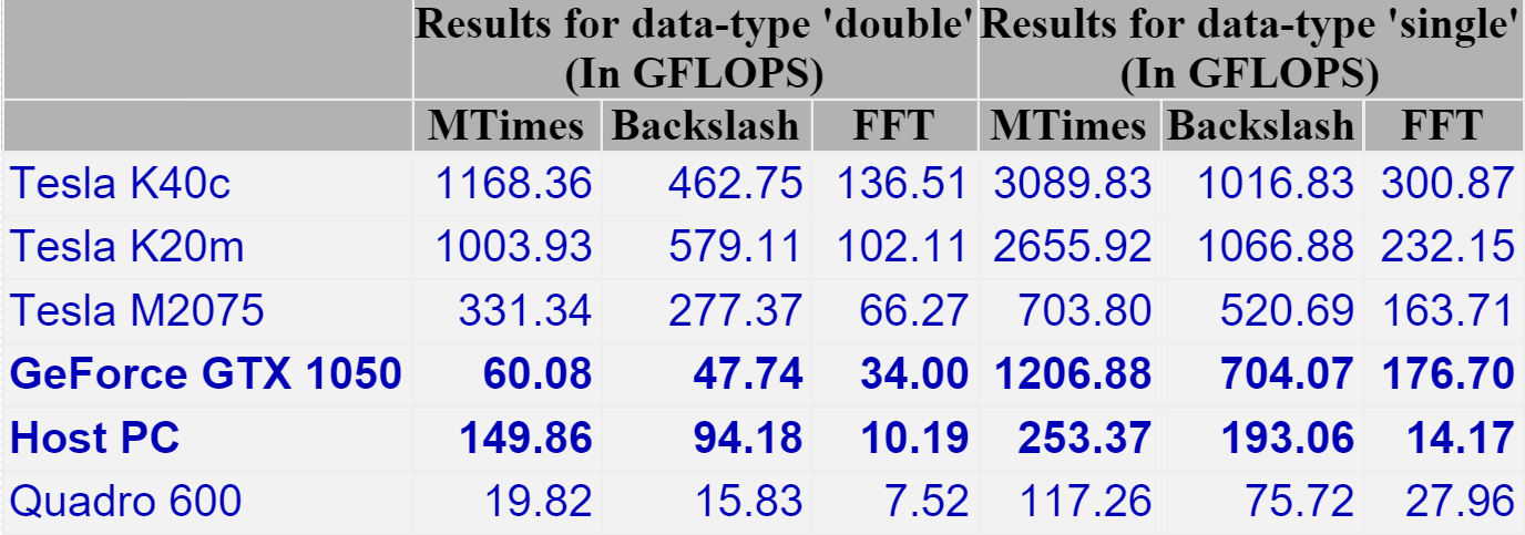
I last did this for my Retina MacBook Pro and am happy to see that the numbers are better across the board. The standout figure for me is the 1206 Gflops (That’s 1.2 Teraflops!) of single precision performance for Matrix-Matrix Multiply.
That figure of 1.2 Teraflops rang a bell for me and it took me a while to realise why…..
My laptop vs Manchester University’s old HPC system – Horace
Old timers like me (I’m almost 40) like to compare modern hardware with bygone supercomputers (1980s Crays vs mobile phones for example) and we know we are truly old when the numbers coming out of laptop benchmarks match the peak theoretical performance of institutional HPC systems we actually used as part of our career.
This has now finally happened to me! I was at the University of Manchester when it commissioned a HPC service called Horace and I was there when it was switched off in 2010 (only 6 and a bit years ago!). It was the University’s primary HPC service with a support team, helpdesk, sysadmins…the lot. The specs are still available on Manchester’s website:
- 24 nodes, each with 8 cores giving 192 cores in total.
- Each core had a theoretical peak compute performance of 6.4 double precision Gflop/s
- So a node had a theoretical peak performance of 51.2 Gflop/s
- The whole thing could theoretically manage 1.2 Teraflop/s
- It had four special ‘high memory’ nodes with 32Gb RAM each
Good luck getting that 1.2 Teraflops out of it in practice!
I get a big geek-kick out of the fact that my new laptop has the same amount of RAM as one of these ‘big memory’ nodes and that my laptop’s double precision CPU performance is on par with the combined power of 3 of Horace’s nodes. Furthermore, my laptop’s GPU can just about manage 1.2 Teraflop/s of single precision performance in MATLAB — on par with the total combined power of the HPC system*.
* (I know, I know….Horace’s numbers are for double precision and my GPU numbers are single precision — apples to oranges — but it still astonishes me that the headline numbers are the same — 1.2 Teraflops).
I work at The University of Sheffield where I am one of the leaders of the new Research Software Engineering function. One of the things that my group does is help people make use of Sheffield’s High Performance Computing cluster, Iceberg.
Iceberg is a heterogenous system with around 3440 CPU cores and a sprinkling of GPUs. It’s been in use for several years and has been upgraded a few times over that period. It’s a very traditional HPC system that makes use of Linux and a variant of Sun Grid Engine as the scheduler and had served us well.

A while ago, the sysadmin pointed me to a goldmine of a resource — Iceberg’s accounting log. This 15 Gigabyte file contains information on every job submitted since July 2009. That’s more than 7 years of the HPC usage of 3249 users — over 46 million individual jobs.
The file format is very straightforward. There’s one line per job and each line consists of a set of colon separated fields. The first few fields look like something like this:
long.q:node54.iceberg.shef.ac.uk:el:abc07de:
The username is field 4 and the number of slots used by the job is field 35. On our system, slots correspond to CPU cores. If you want to run a 16 core job, you ask for 16 slots.
With one line of awk, we can determine the maximum number of slots ever requested by each user.
gawk -F: '$35>=slots[$4] {slots[$4]=$35};END{for(n in slots){print n, slots[n]}}' accounting > ./users_max_slots.csv
As a quick check, I grepped the output file for my username and saw that the maximum number of cores I’d ever requested was 20. I ran a 32 core MPI ‘Hello World’ job, reran the line of awk and confirmed that my new maximum was 32 cores.
There are several ways I could have filtered the number of users but I was having awk lessons from David Jones so let’s create a new file containing the users who have only ever requested 1 slot.
gawk -F: '$35>=slots[$4] {slots[$4]=$35};END{for(n in slots){if(slots[n]==1){print n, slots[n]}}}' accounting > users_where_max_is_one_slot.csv
Running wc on these files allows us to determine how many users are in each group
wc users_max_slots.csv

3250  6498 32706 users_max_slots.csv
One of those users turned out to be a blank line so 3249 usernames have been used on Iceberg over the last 7 years.
wc users_where_max_is_one_slot.csv
2393  4786 23837 users_where_max_is_one_slot.csv
That is, 2393 of our 3249 users (just over 73%) over the last 7 years have only ever run 1 slot, and therefore 1 core, jobs.
High Performance?
So 73% of all users have only ever submitted single core jobs. This does not necessarily mean that they have not been making use of parallelism. For example, they might have been running job arrays – hundreds or thousands of single core jobs performing parameter sweeps or monte carlo simulations.
Maybe they were running parallel codes but only asked the scheduler for one core. In the early days this would have led to oversubscribed nodes, possibly up to 16 jobs, each trying to run 16 cores.These days, our sysadmin does some voodoo to ensure that jobs can only use the number of cores that have been requested, no matter how many threads their code is spawning. Either way, making this mistake is not great for performance.
Whatever is going on, this figure of 73% is surprising to me!
Thanks to David Jones for the awk lessons although if I’ve made a mistake, it’s all my fault!
Update (11th Jan 2017)
UCL’s Ian Kirker took a look at the usage of their general purpose cluster and found that 71.8% of their users have only ever run 1 core jobs. https://twitter.com/ikirker/status/819133966292807680
The High Performance Computing system at University of Sheffield has several different file systems available to it. We have:-
- /fastdata – A lustre-based, shared filesystem with hundreds of terabytes of space. No backup. No quota.
- /data – An NFS file system where each user has access to 100Gb of storage. Back-ups go back 7 days.
- /home – An NFS file system where each user has 10Gb. Backed up over 28 days. Mirrored.
- /scratch – Local disk on each worker node. No back up. Uses ext4.
Lots of options with differing amounts of space, back-up policy and, as I’m about to demonstrate, performance characteristics. I suspect that many other HPC systems have a similar set up.
On our system, it’s very tempting to do everything in /fastdata. There’s lots of space, no quota, readable from all worker nodes simultaneously — good times! I try to encourage people to think about what they are doing, however. Bad things can happen if the lustre filesystem is hammered too much. Also, there can be a huge difference in performance for some operations across different filesystems.
Let’s take an example. I want to download and untar gcc 4.9.2. How long does that take on the three different filesystems?
On the scratch directory of a worker node
cd \scratch
mkdir testing123
cd testing123
wget ftp://ftp.mirrorservice.org/sites/sourceware.org/pub/gcc/releases/gcc-4.9.2/gcc-4.9.2.tar.gz
time tar xfz ./gcc-4.9.2.tar.gz

real    0m6.237s
user    0m5.302s
sys 0m3.033s
On the lustre filesystem
cd /fastdata/
mkdir testing123
cd testing123
wget ftp://ftp.mirrorservice.org/sites/sourceware.org/pub/gcc/releases/gcc-4.9.2/gcc-4.9.2.tar.gz
time tar xfz ./gcc-4.9.2.tar.gz

real    7m18.170s
user    0m6.751s
sys 0m56.802s
On the NFS filesystem
cd /data/myusername
mkdir testing123
cd testing123
wget ftp://ftp.mirrorservice.org/sites/sourceware.org/pub/gcc/releases/gcc-4.9.2/gcc-4.9.2.tar.gz
time tar xfz ./gcc-4.9.2.tar.gz

real	16m37.343s
user	0m6.052s
sys	0m23.438s
For this particular operation, there is a two orders of magnitude difference between the worst and the best option.
I’m not an expert in filesystems and I have no idea what’s causing these differences or if I’d see a similar speed difference given a different file operation. I currently have no interest in doing a robust set of benchmarks. The point I’m making is that if you are using a system that has multiple filesystems it may be worth checking if there’s an advantage to using one over the other for your particular use case.
I was sat in a meeting recently where people were discussing High Performance Computing options. Someone had found some money down the back of the sofa and asked the rest of us how we’d spend it if it were ours (For the record, I wanted some big-memory nodes — 512Gb RAM minimum).
Halfway through the meeting someone asked about the parallel filesystem in use on Sheffield’s HPC systems and I answered Lustre — not expecting any further comment. I don’t know much about parallel I/O systems but I do know that all of the systems I have access to make use of Lustre. Sheffield’s Iceberg, Manchester’s Computational Shared Facility and the UK National supercomputer, Archer to name three. The Wikipedia page for Lustre suggests that it is very widely used in the HPC community worldwide.
I was surprised, then, when this comment was met with derision from some in the room. One person remarked ‘It’s a bit…um…classic..isn’t it?’, giving the impression that it was old and outdated. There was not much love for dear old Lustre it seemed!
There was no time in this meeting for me ask ‘What’s wrong with it then? Works fine for me!’so I did what I often do in times like this, I asked twitter:
Q for HPC followers. Is there anything wrong with using Lustre? Just been in a meeting where it was mocked as ‘classic’.
— Mike Croucher (@walkingrandomly) April 12, 2016
I found the responses to be very instructive so thought I would share them here. Here’s a comment from Ben Waugh
@walkingrandomly Lustre failures seem to be the main cause of downtime in my limited experience of large HPC systems.
— Ben Waugh (@benwaughuk) April 12, 2016
Not a great start! I’ve been hit by Lustre downtime too but, since I’m not a sysadmin, I haven’t got a genuine sense of how big a problem it is. It happens often enough that I’m aware of it but not so often that I feel the need to worry about it. Looking after large HPC systems is difficult and when one attempts to do do something difficult, the occasional failure is inevitable.
It seems that configuration might play a part in stability and performance. Peter Van Heusden kicked off with
@walkingrandomly Depending on the configuration can lack resilience, but is still standard HPC parallel FS.
— Peter van Heusden (@pvanheus) April 12, 2016
Adrian Jackson , Research Architect, HPC and Parallel Programmer, is thinking along similar lines.
@walkingrandomly 1/2 Yes, for a long time the metadata servers have not kept up, meaning you can destroy it with lots of small files
— Adrian Jackson (@adrianjhpc) April 12, 2016
@walkingrandomly 2/2 Although I believe this is being fixed in a variety of ways.
— Adrian Jackson (@adrianjhpc) April 12, 2016
@walkingrandomly Also, the default settings often don’t give best large scale performance, but that’s a matter of configuration
— Adrian Jackson (@adrianjhpc) April 12, 2016
Adrian also followed up with an interesting report on Performance of Parallel IO on ARCHER from June 2015. Thanks Adrian!
Glen K Lockwood is a Computational scientist specialising in I/O platforms at @NERSC, the flagship computing centre for the U.S. Dept. of Energy’s Office of Science. Glen has this insight,
@eoinbrazil @walkingrandomly Lustre just gets trashed because everyone uses it (because of its cost). Parallel file systems all misbehave
— Glenn K. Lockwood (@glennklockwood) April 12, 2016
I like this comment because it fits with my own, much less experienced, view of the parallel I/O world. A classic demonstration of confirmation bias perhaps but I see this thought pattern in a lot of areas. The pattern looks like this:
It’s hard to do ‘thing’. Most smart people do ‘thing’ with ‘foo’ and, since ‘thing’ is hard, many people have experienced problems with ‘foo’. Hence, people bash ‘foo’ a lot. ‘foo’ sucks!
Alternatives exist of course but there may be trade-offs. Here’s Mark Basham, software scientist @diamondlightsou in the UK.
@walkingrandomly we use it at Diamond for several of our file systems. GPFS is a bit better, but a lot more costly.
— Mark Basham (@basham_mark) April 12, 2016
I’ll give the final word to Nick Holway who sums up how I feel about parallel storage from a user’s point of view.
@walkingrandomly I like my HPC storage to be "classic" and also rather "boring"
— Nick Holway (@nickholway) April 12, 2016
I hang out with a lot of people who work in the field of High Performance Computing (HPC) and learned long ago that a great conversation starter when in a room full of HPC experts is to ask the question ‘So…what IS High Performance Computing’ and then offer some opinion of my own. This apparently simple question can lead to some very heated debates!
I’m feeling in a curious mood and am wondering if this would work as a conversation starter for a blog post. So, here goes….
‘What IS High Performance Computing? I think it’s anything that requires more computational resources (memory, disk, CPU/GPU) than is available on a typical half-decent laptop or desktop’
What’s your view? Comments are open!
Environment modules are widely used in the High Performance Computing (HPC) world where sysadmins need to install dozens, or maybe hundreds of potentially conflicting applications, libraries and compilers on multi-user machines. The University of Manchester’s Computational Shared Facility (CSF), for example, makes extensive use of environment modules and would be extremely difficult to run without them.
Once the sysadmin has correctly installed an application (MATLAB 2014a say) and set up the corresponding module file, making it available to your shell is as easy as doing
module load apps/binapps/matlab/R2014a
Unloading the module is just as easy
module unload apps/binapps/matlab/R2014a
On a heavily used, multi-user system environment modules are invaluable! Every user can have whatever compilers, libraries and applications they like — they just load and unload whatever they need from the huge selection supported by their ever-friendly sysadmins.
Environment modules on Ubuntu
I needed to install environment modules on a VM running Ubuntu 14.04 for my own use. I found a very nice setup guide at http://www.setuptips.com/unix/setup-environment-modules-on-ubuntu/ but it didn’t work. On attempting to compile, I got the error message
cmdModule.c:644:15: error: 'Tcl_Interp' has no member named 'errorLine'
This is a known bug in version 3.2.9c of environment modules and has a work-around.
I also found a set up guide at http://nickgeoghegan.net/linux/installing-environment-modules which had some useful advice on configuration..
Combining information from these sources, I managed to get a working install. Here are the steps I did in full for a clean Ubuntu 14.04 image
#Install the tcl development package
sudo apt-get install tcl-dev

#Make the directories where my modules and packages are going to live
sudo mkdir /opt/modules
sudo mkdir /opt/packages

#Get the source code. This was the most up to date version as of 25th Feb 2015
wget http://downloads.sourceforge.net/project/modules/Modules/modules-3.2.9/modules-3.2.9c.tar.gz

#unpack and enter source directory
tar xvzf modules-3.2.9c.tar.gz
cd modules-3.2.9

#Configure using the workaround and selecting my module folder
CPPFLAGS="-DUSE_INTERP_ERRORLINE" ./configure --with-module-path=/opt/modules/

#make and install
make
sudo make install

#Edit the modulefiles path. Comment out all lines starting /usr so that only /opt/modules is used
sudo sed -i 's~^/usr~#/usr~' /usr/local/Modules/3.2.9/init/.modulespath

#Configure the shell to use modules
sudo tee /etc/profile.d/modules.sh > /dev/null << 'EOF'
#----------------------------------------------------------------------#
# system-wide profile.modules #
# Initialize modules for all sh-derivative shells #
#----------------------------------------------------------------------#
trap "" 1 2 3

MODULES=/usr/local/Modules/3.2.9

case "$0" in
-bash|bash|*/bash) . $MODULES/init/bash ;;
-ksh|ksh|*/ksh) . $MODULES/init/ksh ;;
-sh|sh|*/sh) . $MODULES/init/sh ;;
*) . $MODULES/init/sh ;; # default for scripts
esac

trap - 1 2 3
EOF

#Add modules to your .bashrc file
echo '#For modules' >> ~/.bashrc
echo '. /etc/profile.d/modules.sh' >> ~/.bashrc
That takes care of the basic setup but modules is pretty useless at this stage. To make it useful, you need to install some extra software and the corresponding module file.
Installing a module file for Anaconda Python 2.1
This is a really simple example of how to set up a basic module file
I downloaded and installed Anaconda Python 2.1 to /opt/packages and created a file called anaconda2.1 in /opt/modules containing the following
#%Module1.0
proc ModulesHelp { } {
global dotversion

puts stderr "\tAnaconda Python 2.1 providing Python 2.7.8"
}

module-whatis "Anaconda Python 2.1"
prepend-path PATH /opt/packages/anaconda/bin
Now, when I do the command
module avail
I get
-------------------------- /opt/modules/ ---------------------------
anaconda2.1
I can load my anaconda2.1 module with the command
module load anaconda2.1
Now, when I type python at the command prompt, I’ll be using Anaconda’s python rather than the system python. Once I’m done, I can unload with
module unload anaconda2.1
This example is so trivial it’s almost not worth it — modules really come into their own when you need to support loads of compilers and corresponding libraries. There’s an example using gcc at http://nickgeoghegan.net/linux/installing-environment-modules.
I work at The University of Manchester as part of IT Service’s Research Support department. This month, I was given the task of editing the newsletter that we send out to the academics we serve.
For me, this month’s highlights include the fact that our Condor Pool (which I help build and run) has now delivered over 20 million CPU hours to academics at Manchester by making use of desktop PCs around campus. Another HPC system we have at Manchester is our Computational Shared Facility which is jointly funded by the University and all of the research groups who use it. This system has just seen the installation of its 6000-th CPU core.
Other news includes the Greater Manchester Data Dive, an AGM for Research Software Engineers, Image based modelling and more.
If you are interested in seeing the sort of thing we get up to, check out this months newsletter at http://documents.manchester.ac.uk/DocuInfo.aspx?DocID=20995
I am having a friendly argument with a colleague over how you calculate the peak number of floating operations per second (flops) for devices that support Fused Multiply Add (FMA). The FMA operation is d=a+b*c, an operation that can be done in one cycle on devices that support it.
I say that an FMA operation is two flops, he says it’s one. So, when I calculate the theoretical peak of a device I get twice the value he does. So, what do you think..is FMA one flop or two?
Intel have finally released the Xeon Phi – an accelerator card based on 60 or so customised Intel cores to give around a Teraflop of double precision performance. That’s comparable to the latest cards from NVIDIA (1.3 Teraflops according to http://www.theregister.co.uk/2012/11/12/nvidia_tesla_k20_k20x_gpu_coprocessors/) but with one key difference—you don’t need to learn any new languages or technologies to take advantage of it (although you can do so if you wish)!
The Xeon Phi uses good, old fashioned High Performance Computing technologies that we’ve been using for years such as OpenMP and MPI. There’s no need to completely recode your algorithms in CUDA or OpenCL to get a performance boost…just a sprinkling of OpenMP pragmas might be enough in many cases. Obviously it will take quite a bit of work to squeeze every last drop of performance out of the thing but this might just be the realisation of ‘personal supercomputer’ we’ve all been waiting for.
Here are some links I’ve found so far — would love to see what everyone else has come up with. I’ll update as I find more
- http://www.theregister.co.uk/2012/11/12/intel_xeon_phi_coprocessor_launch/ (Includes pricing and some benchmarks)
- http://www.streamcomputing.eu/blog/2012-11-12/intels-answer-to-amd-and-nvidia-the-xeon-phi-5110p/ (lots of details, programming models and comparisons with GPUs)
- http://software.intel.com/en-us/blogs/2012/11/12/introducing-opencl-12-for-intel-xeon-phi-coprocessor (Intel’s OpenCL works on Xeon Phi)
- http://www.hpcwire.com/hpcwire/2012-11-12/nag_delivers_numerical_software_to_xeon_phi.html (My favourite numerical library has already been ported to the Phi)
I also note that the Xeon Phi uses AVX extensions but with a wider vector width of 512 bytes so if you’ve been taking advantage of that technology in your code (using one of these techniques perhaps) you’ll reap the benefits there too.
I, for one, am very excited and can’t wait to get my hands on one! Thoughts, comments and links gratefully received!